Algorithms For Small World Networks Anurag singh Outlines

Algorithms For Small World Networks Anurag singh

Outlines Introduction Characteristics of Small World Network Literature survey Structural Models Algorithmic side of Kleinberg’s model Applications of Kleinberg’s decentralized algorithm � � �

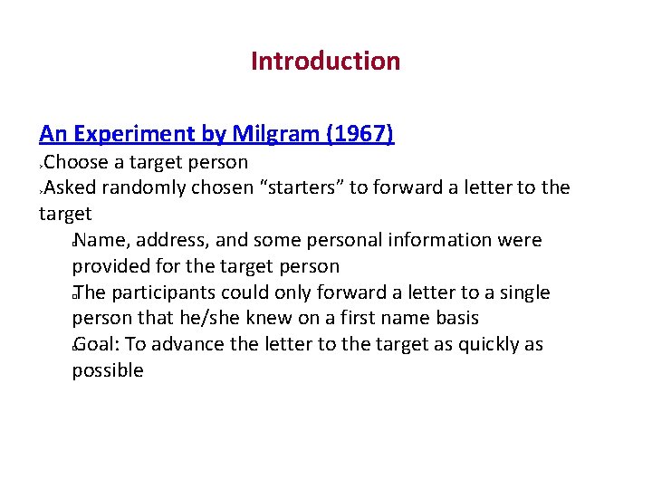
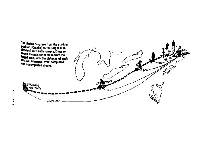
Introduction An Experiment by Milgram (1967) Choose a target person Asked randomly chosen “starters” to forward a letter to the target Name, address, and some personal information were provided for the target person The participants could only forward a letter to a single person that he/she knew on a first name basis Goal: To advance the letter to the target as quickly as possible � � �

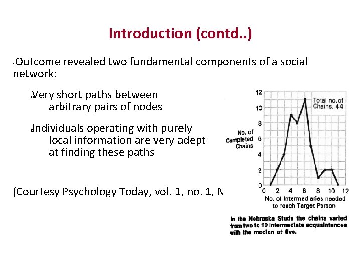
Introduction (contd. . ) Outcome revealed two fundamental components of a social network: Very short paths between arbitrary pairs of nodes � Individuals operating with purely local information are very adept at finding these paths � (Courtesy Psychology Today, vol. 1, no. 1, May 1967, pp 61‐ 67)

Introduction (contd. . ) Outcome revealed two fundamental components of a social network: Very short paths between arbitrary pairs of nodes � Individuals operating with purely local information are very adept at finding these paths � ( Psychology Today, vol. 1, no. 1, May 1967, pp 61‐ 67)

Introduction (contd. . ) Outcome revealed two fundamental components of a social network: Very short paths between arbitrary pairs of nodes � Individuals operating with purely local information are very adept at finding these paths � (Courtesy Psychology Today, vol. 1, no. 1, May 1967, pp 61‐ 67)

Structural Models Regular networks Random networks Small‐world networks Scale free networks

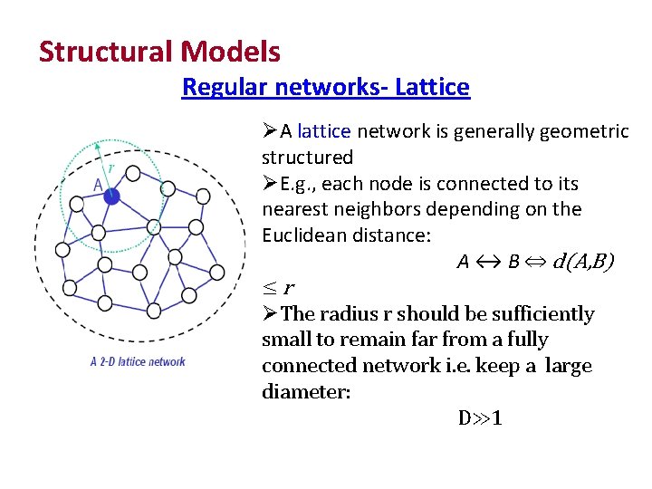
Structural Models Regular networks- Lattice A lattice network is generally geometric structured E. g. , each node is connected to its nearest neighbors depending on the Euclidean distance: A ↔ B ⇔ d(A, B) ≤r The radius r should be sufficiently small to remain far from a fully connected network i. e. keep a large diameter: D≫ 1

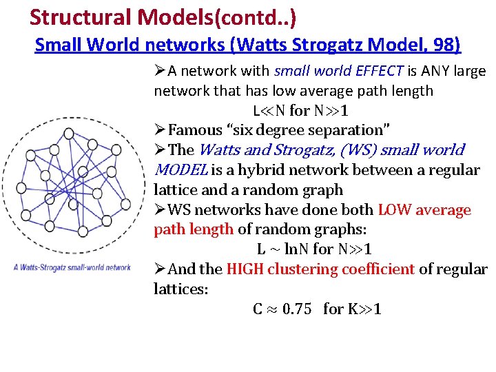
Structural Models(contd. . ) Small World networks (Watts Strogatz Model, 98) A network with small world EFFECT is ANY large network that has low average path length L≪N for N≫ 1 Famous “six degree separation” The Watts and Strogatz, (WS) small world MODEL is a hybrid network between a regular lattice and a random graph WS networks have done both LOW average path length of random graphs: L ∼ ln. N for N≫ 1 And the HIGH clustering coefficient of regular lattices: C ≈ 0. 75 for K≫ 1

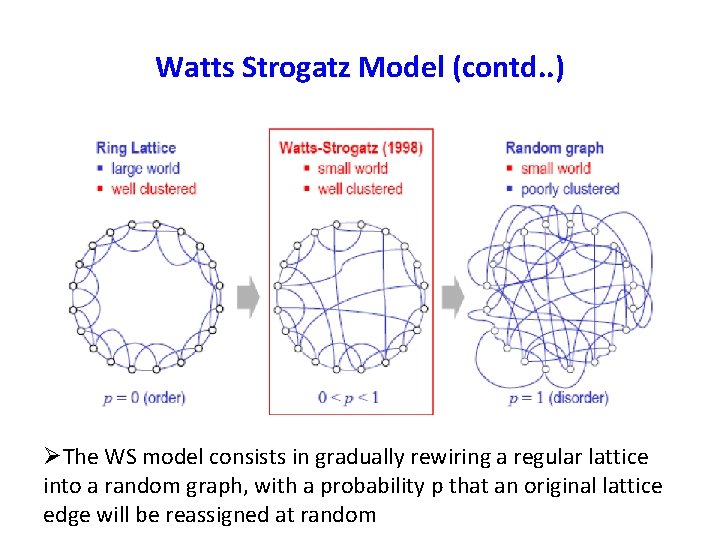
Watts Strogatz Model (contd. . ) The WS model consists in gradually rewiring a regular lattice into a random graph, with a probability p that an original lattice edge will be reassigned at random

Watts Strogatz Model (contd. . ) The WS model consists in gradually rewiring a regular lattice into a random graph, with a probability p that an original lattice edge will be reassigned at random

Watts Strogatz Model (contd. . ) The WS model consists in gradually rewiring a regular lattice into a random graph, with a probability p that an original lattice edge will be reassigned at random

Structural Models(contd. . ) Newman and Watts model, 99

Algorithmic issues • So, The short path exists. (Structurally) • But how can we find it? • If we want the shortest path “flooding” of the network � • Milgram’s experiment “tunneling” through the network how to make decentralized routing so effective? � �

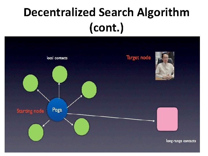
Decentralized Search Algorithm • starting node s • target node t • seek to pass a message from s to t, by advancing the message along edges • In each step, the current message holder v has knowledge of: the underlying grid structure the location of the target t on the grid certain global “reference frames” its own long‐range contact � � � • The short path is unknown!

Decentralized Search Algorithm (cont. )

Decentralized Search Algorithm (cont. ) • Delivery time: expected number of step required to reach the target

The first result is negative • The delivery time of any decentralized algorithm in the grid‐based model is Ω(n 2/3) (Kleinberg, J. , The small‐world phenomenon: An algorithmic perspective. Proceedings of the 32 nd Annual Symposium on Theory of Computing (2000)) � • It’s not polylogarithmic in n. • But it’s not the end of the story.

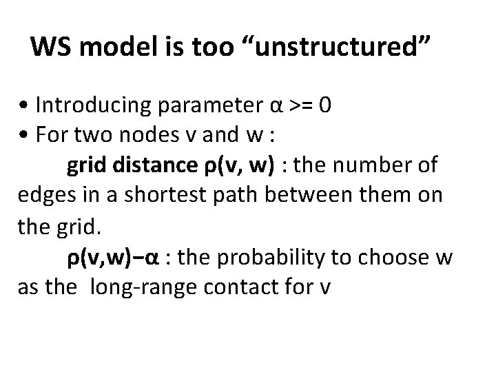
WS model is too “unstructured” • Introducing parameter α >= 0 • For two nodes v and w : grid distance ρ(v, w) : the number of edges in a shortest path between them on the grid. ρ(v, w)−α : the probability to choose w as the long‐range contact for v

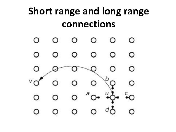
Short range and long range connections

WS model is too “unstructured”(cont. ) • Theorem. (a)For 0≤ α < 2, the delivery time of any decentralized search algorithm in the grid‐based model is Ω (n(2‐ α)/3). • (b) For α=2, there is a decentralized algorithm with delivery time O(log 2 n). • (c)For α>2, the delivery time of any decentralized algorithm in the grid‐based model is Ω(n(α‐ 2)/(α‐ 1)) Kleinberg, J. , The small‐world phenomenon: An algorithmic perspective. Proceedings of the 32 nd Annual Symposium on Theory of Computing (2000) � • α too small : too random(uniformly) • α too large : not random enough

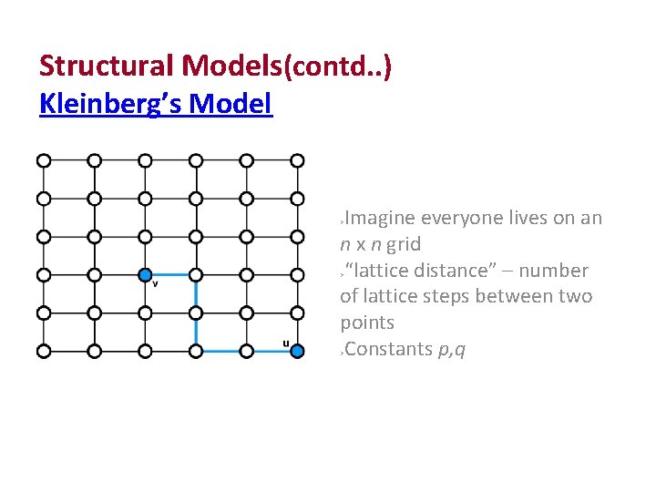
Structural Models(contd. . ) Kleinberg’s Model Imagine everyone lives on an n x n grid “lattice distance” – number of lattice steps between two points Constants p, q

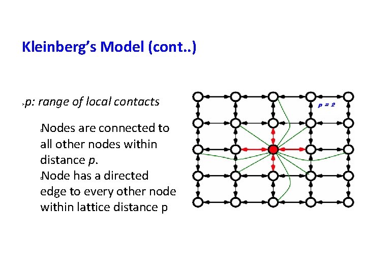
Kleinberg’s Model (cont. . ) p: range of local contacts Nodes are connected to all other nodes within distance p. Node has a directed edge to every other node within lattice distance p � �

Kleinberg’s Model (cont. . ) p: range of local contacts Nodes are connected to all other nodes within distance p. Node has a directed edge to every other node within lattice distance p � �

Kleinberg’s Model (cont. . ) p: range of local contacts Nodes are connected to all other nodes within distance p. Node has a directed edge to every other node within lattice distance p � �

Kleinberg’s Model (cont. . ) p: range of local contacts Nodes are connected to all other nodes within distance p. Node has a directed edge to every other node within lattice distance p � �

(Courtesy Psychology Today, vol. 1, no. 1, May 1967, pp 61‐ 67) Slide 3

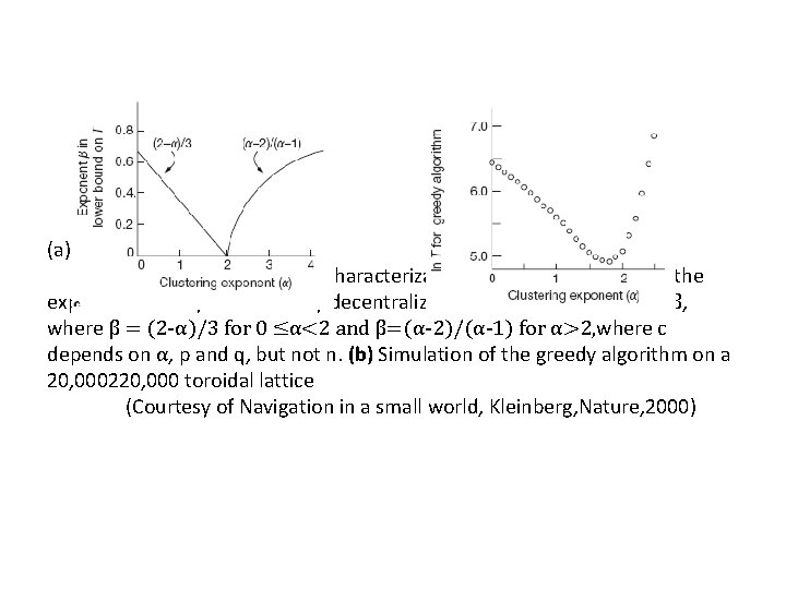
(a) (b) (a)Lower bound from characterization theorem: when a ≠ 2, the expected delivery time T of any decentralized algorithm satisfies T≥cnβ, where β = (2 -α)/3 for 0 ≤α<2 and β=(α-2)/(α-1) for α>2, where c depends on α, p and q, but not n. (b) Simulation of the greedy algorithm on a 20, 000220, 000 toroidal lattice (Courtesy of Navigation in a small world, Kleinberg, Nature, 2000)

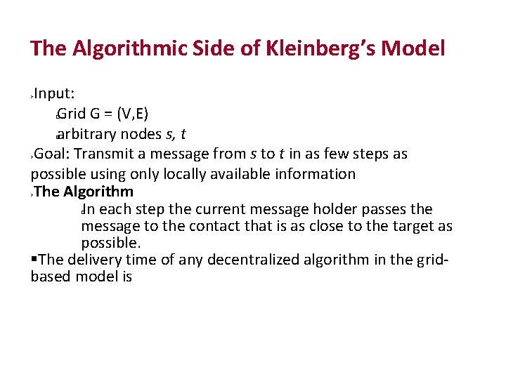
Kleinberg’s Model (cont. . ) Pr [u has v as its long range contact] : Infinite family of networks: r = 0: each node’s long‐range contacts are chosen independently of its position on the grid As r increases, the long range contacts of a node become clustered in its vicinity on the grid. � �

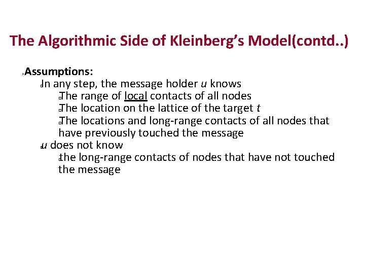
The Algorithmic Side of Kleinberg’s Model Input: Grid G = (V, E) arbitrary nodes s, t Goal: Transmit a message from s to t in as few steps as possible using only locally available information The Algorithm In each step the current message holder passes the message to the contact that is as close to the target as possible. The delivery time of any decentralized algorithm in the grid‐ based model is � � �

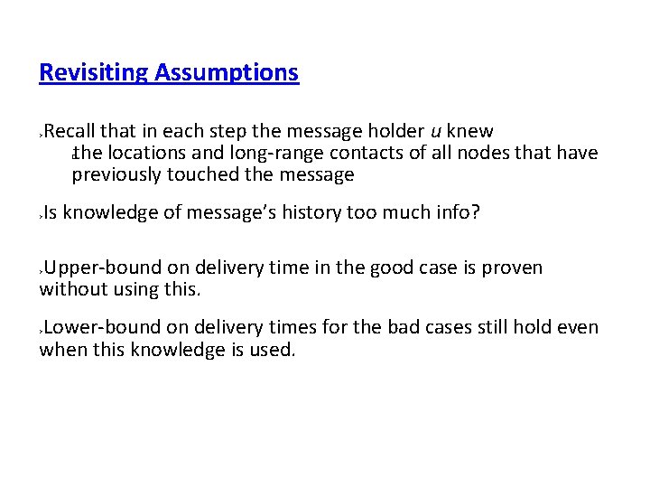
The Algorithmic Side of Kleinberg’s Model(contd. . ) Assumptions: In any step, the message holder u knows The range of local contacts of all nodes The location on the lattice of the target t The locations and long‐range contacts of all nodes that have previously touched the message u does not know the long‐range contacts of nodes that have not touched the message � � �

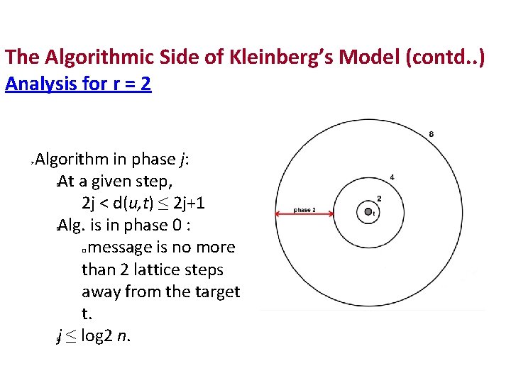
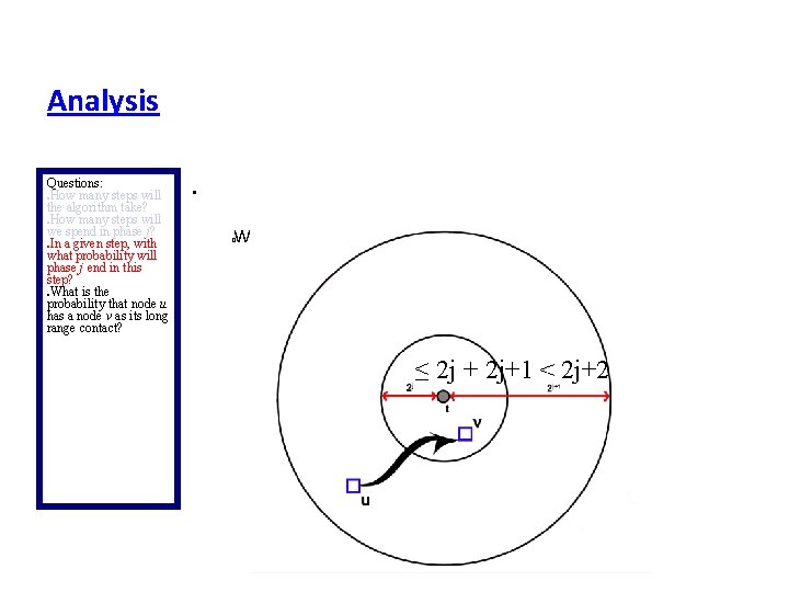
The Algorithmic Side of Kleinberg’s Model (contd. . ) Analysis for r = 2 Algorithm in phase j: At a given step, 2 j < d(u, t) ≤ 2 j+1 Αlg. is in phase 0 : message is no more than 2 lattice steps away from the target t. j ≤ log 2 n. � �

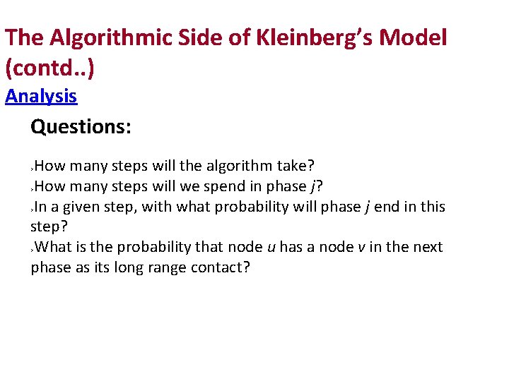
The Algorithmic Side of Kleinberg’s Model (contd. . ) Analysis Questions: How many steps will the algorithm take? How many steps will we spend in phase j? In a given step, with what probability will phase j end in this step? What is the probability that node u has a node v in the next phase as its long range contact?

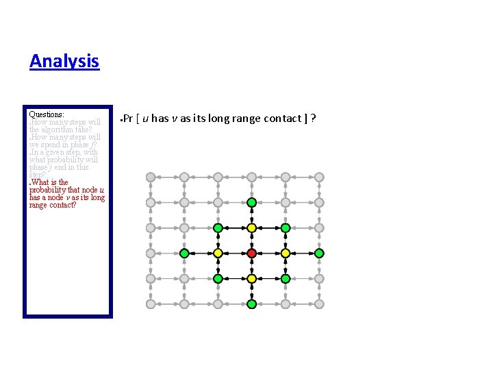
Analysis Questions: How many steps will the algorithm take? How many steps will we spend in phase j? In a given step, with what probability will phase j end in this step? What is the probability that node u has a node v as its long range contact? Pr [ u has v as its long range contact ] ?

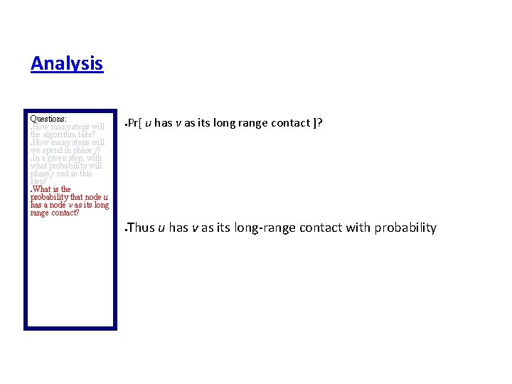
Analysis Questions: How many steps will the algorithm take? How many steps will we spend in phase j? In a given step, with what probability will phase j end in this step? What is the probability that node u has a node v as its long range contact? Pr[ u has v as its long range contact ]? Thus u has v as its long‐range contact with probability

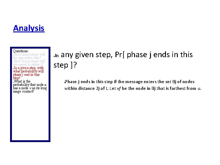
Analysis Questions: How many steps will the algorithm take? How many steps will we spend in phase j? In a given step, with what probability will phase j end in this step? What is the probability that node u has a node v as its long range contact? any given step, Pr[ phase j ends in this step ]? In Phase j ends in this step if the message enters the set Bj of nodes within distance 2 j of t. Let vf be the node in Bj that is farthest from u. �

Analysis Questions: How many steps will the algorithm take? How many steps will we spend in phase j? In a given step, with what probability will phase j end in this step? What is the probability that node u has a node v as its long range contact? What is d[(u, vf)]? � ≤ 2 j + 2 j+1 < 2 j+2

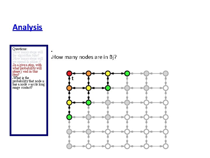
Analysis Questions: How many steps will the algorithm take? How many steps will we spend in phase j? In a given step, with what probability will phase j end in this step? What is the probability that node u has a node v as its long range contact? How many nodes are in Bj?

Analysis Questions: How many steps will the algorithm take? How many steps will we spend in phase j? In a given step, with what probability will phase j end in this step? What is the probability that node u has a node v as its long range contact? In any given step, Pr[ phase j ends in this step ]? Pr[ u has a long‐range contact in Bj ]? �

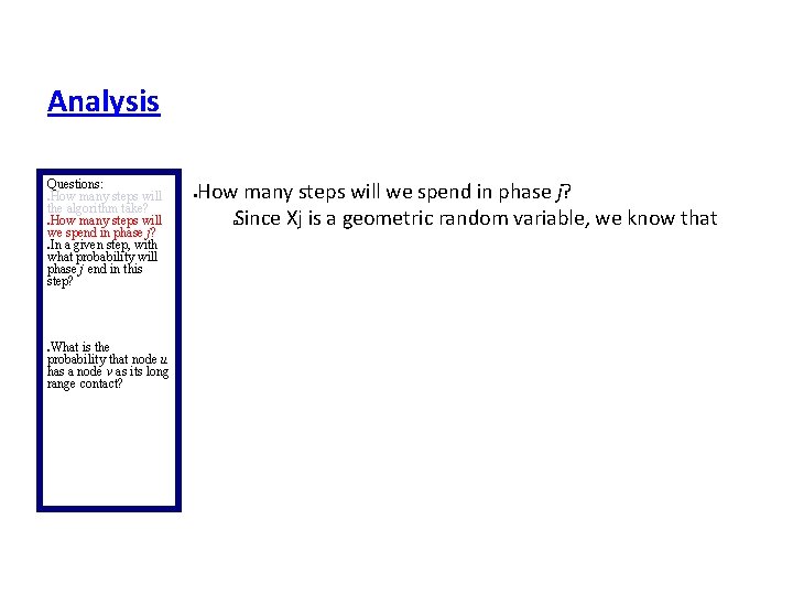
Analysis Questions: How many steps will the algorithm take? How many steps will we spend in phase j? In a given step, with what probability will phase j end in this step? What is the probability that node u has a node v as its long range contact? How many steps will we spend in phase j? Let Xj be a random variable denoting the number of steps spent in phase j. Xj is a geometric random variable with a probability of success at least � �

Analysis Questions: How many steps will the algorithm take? How many steps will we spend in phase j? In a given step, with what probability will phase j end in this step? What is the probability that node u has a node v as its long range contact? How many steps will we spend in phase j? Since Xj is a geometric random variable, we know that �

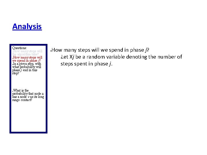
Analysis Questions: How many steps will the algorithm take? How many steps will we spend in phase j? In a given step, with what probability will phase j end in this step? What is the probability that node u has a node v as its long range contact? How many steps will we spend in phase j? Let Xj be a random variable denoting the number of steps spent in phase j. �

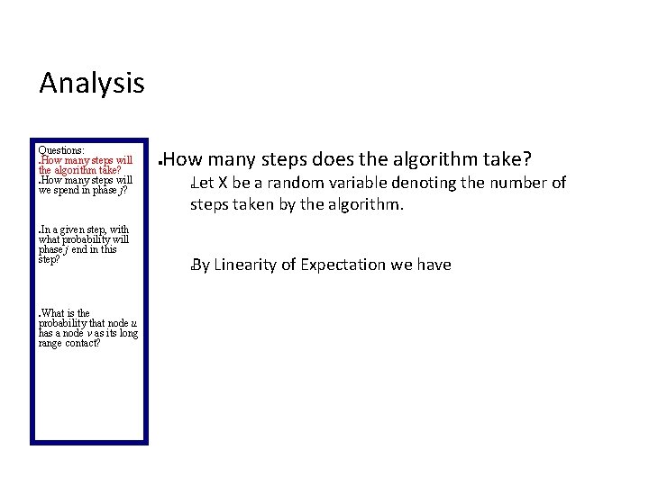
Analysis Questions: How many steps will the algorithm take? How many steps will we spend in phase j? In a given step, with what probability will phase j end in this step? How many steps does the algorithm take? Let X be a random variable denoting the number of steps taken by the algorithm. � By Linearity of Expectation we have � What is the probability that node u has a node v as its long range contact?

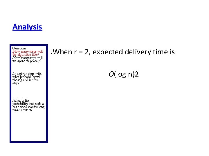
Analysis Questions: How many steps will the algorithm take? How many steps will we spend in phase j? When r = 2, expected delivery time is In a given step, with what probability will phase j end in this step? What is the probability that node u has a node v as its long range contact? O(log n)2

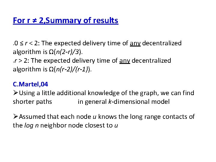
For r ≠ 2, Summary of results 0 ≤ r < 2: The expected delivery time of any decentralized algorithm is Ω(n(2 -r)/3). r > 2: The expected delivery time of any decentralized algorithm is Ω(n(r-2)/(r-1)). C. Martel, 04 Using a little additional knowledge of the graph, we can find shorter paths in general k‐dimensional model Assumed that each node u knows the long range contacts of the log n neighbor node closest to u

Revisiting Assumptions Recall that in each step the message holder u knew the locations and long‐range contacts of all nodes that have previously touched the message � Is knowledge of message’s history too much info? Upper‐bound on delivery time in the good case is proven without using this. Lower‐bound on delivery times for the bad cases still hold even when this knowledge is used.

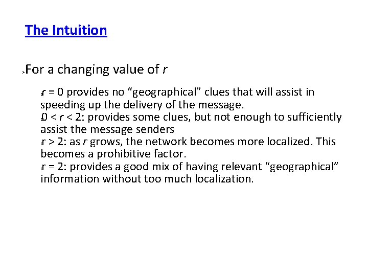
The Intuition For a changing value of r r = 0 provides no “geographical” clues that will assist in speeding up the delivery of the message. 0 < r < 2: provides some clues, but not enough to sufficiently assist the message senders r > 2: as r grows, the network becomes more localized. This becomes a prohibitive factor. r = 2: provides a good mix of having relevant “geographical” information without too much localization. � �

Some Applications Areas P 2 P overlay networks Distributed hashing protocols Security systems in mobile ad hoc networks Hybrid sensor networks Referral systems For computer scientists small world phenomenon is interesting: efficient routing searching

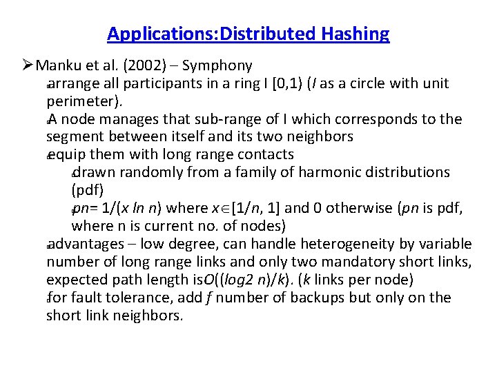
Applications: Distributed Hashing Manku et al. (2002) – Symphony arrange all participants in a ring I [0, 1) (I as a circle with unit perimeter). A node manages that sub‐range of I which corresponds to the segment between itself and its two neighbors equip them with long range contacts drawn randomly from a family of harmonic distributions (pdf) pn= 1/(x ln n) where x [1/n, 1] and 0 otherwise (pn is pdf, where n is current no. of nodes) advantages – low degree, can handle heterogeneity by variable number of long range links and only two mandatory short links, expected path length is. O((log 2 n)/k). (k links per node) for fault tolerance, add f number of backups but only on the short link neighbors. � � � �

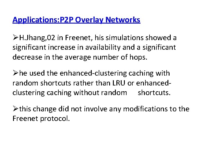
Applications: P 2 P Overlay Networks H. Jhang, 02 in Freenet, his simulations showed a significant increase in availability and a significant decrease in the average number of hops. he used the enhanced‐clustering caching with random shortcuts rather than LRU or enhanced‐ clustering caching without random shortcuts. this change did not involve any modifications to the Freenet protocol.

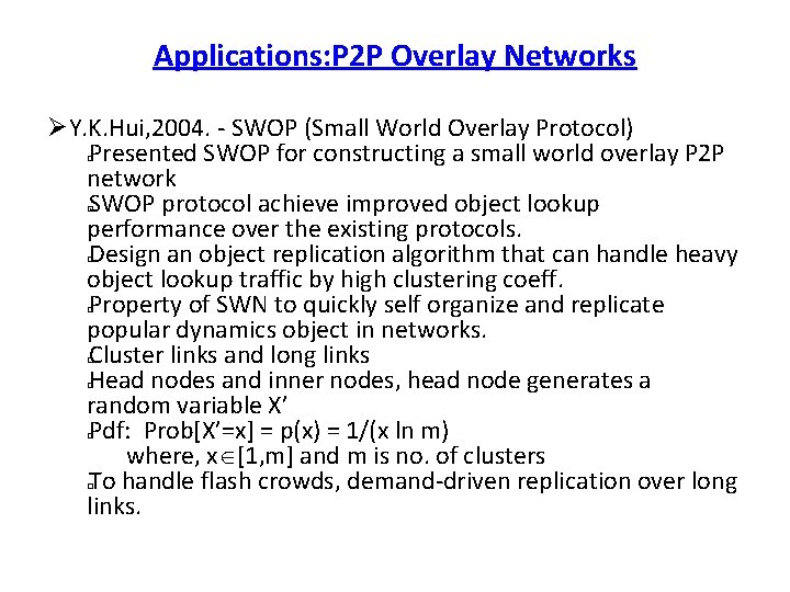
Applications: P 2 P Overlay Networks Y. K. Hui, 2004. ‐ SWOP (Small World Overlay Protocol) Presented SWOP for constructing a small world overlay P 2 P network SWOP protocol achieve improved object lookup performance over the existing protocols. Design an object replication algorithm that can handle heavy object lookup traffic by high clustering coeff. Property of SWN to quickly self organize and replicate popular dynamics object in networks. Cluster links and long links Head nodes and inner nodes, head node generates a random variable X’ Pdf: Prob[X’=x] = p(x) = 1/(x ln m) where, x [1, m] and m is no. of clusters To handle flash crowds, demand‐driven replication over long links. � � � �

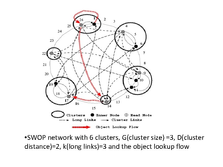
• SWOP network with 6 clusters, G(cluster size) =3, D(cluster distance)=2, k(long links)=3 and the object lookup flow