Algorithms for Map Construction and Comparison Map Construction




![Map Construction Approaches [BE 12] J. Biagioni, J. Eriksson, Map inference in the face Map Construction Approaches [BE 12] J. Biagioni, J. Eriksson, Map inference in the face](https://slidetodoc.com/presentation_image_h2/c8851261d8d36378cd6650fc2cef7703/image-11.jpg)
![Map Construction: More Results • Topological approach on neighborhood complex: [GSBW 11]: Uses Reeb Map Construction: More Results • Topological approach on neighborhood complex: [GSBW 11]: Uses Reeb](https://slidetodoc.com/presentation_image_h2/c8851261d8d36378cd6650fc2cef7703/image-12.jpg)
![Map Construction: Even More Results • Intersection linking [FK 10, KP 12]: First detect Map Construction: Even More Results • Intersection linking [FK 10, KP 12]: First detect](https://slidetodoc.com/presentation_image_h2/c8851261d8d36378cd6650fc2cef7703/image-13.jpg)
![Map Construction [AW 12] Incrementally add one trajectory after another. For each trajectory: 1. Map Construction [AW 12] Incrementally add one trajectory after another. For each trajectory: 1.](https://slidetodoc.com/presentation_image_h2/c8851261d8d36378cd6650fc2cef7703/image-14.jpg)
![Map Construction [AW 12] Incrementally add one trajectory after another. For each trajectory: 1. Map Construction [AW 12] Incrementally add one trajectory after another. For each trajectory: 1.](https://slidetodoc.com/presentation_image_h2/c8851261d8d36378cd6650fc2cef7703/image-16.jpg)
![Map Construction [AW 12] Incrementally add one trajectory after another. For each trajectory: 1. Map Construction [AW 12] Incrementally add one trajectory after another. For each trajectory: 1.](https://slidetodoc.com/presentation_image_h2/c8851261d8d36378cd6650fc2cef7703/image-19.jpg)
![Map Construction [AW 12] Incrementally add one trajectory after another. For each trajectory: 1. Map Construction [AW 12] Incrementally add one trajectory after another. For each trajectory: 1.](https://slidetodoc.com/presentation_image_h2/c8851261d8d36378cd6650fc2cef7703/image-21.jpg)

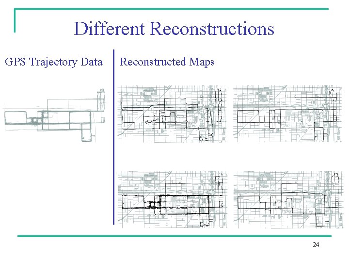

![Average/Mean Curve Given a set f 1, …, fk : [0, 1] R 2 Average/Mean Curve Given a set f 1, …, fk : [0, 1] R 2](https://slidetodoc.com/presentation_image_h2/c8851261d8d36378cd6650fc2cef7703/image-33.jpg)



![Some Results • [CGHS 10]: First algorithm with quality guarantees. Subsamples trajectories Dense point Some Results • [CGHS 10]: First algorithm with quality guarantees. Subsamples trajectories Dense point](https://slidetodoc.com/presentation_image_h2/c8851261d8d36378cd6650fc2cef7703/image-45.jpg)
![Some More Results • [FK 10]: First identify intersections (vertices) using a shape descriptor, Some More Results • [FK 10]: First identify intersections (vertices) using a shape descriptor,](https://slidetodoc.com/presentation_image_h2/c8851261d8d36378cd6650fc2cef7703/image-46.jpg)
![[CGHS 10] Algorithm Steps 1. 2. 3. 4. 5. Compute be-net (subsample to obtain [CGHS 10] Algorithm Steps 1. 2. 3. 4. 5. Compute be-net (subsample to obtain](https://slidetodoc.com/presentation_image_h2/c8851261d8d36378cd6650fc2cef7703/image-47.jpg)

![[AW 12] Incrementally add one trajectory after another. For each trajectory: 1. Use partial [AW 12] Incrementally add one trajectory after another. For each trajectory: 1. Use partial](https://slidetodoc.com/presentation_image_h2/c8851261d8d36378cd6650fc2cef7703/image-57.jpg)
- Slides: 60

Algorithms for Map Construction and Comparison: Map Construction I Carola Wenk Department of Computer Science Tulane University Collaborators: Mahmuda Ahmed, Brittany Fasy, Kyle Hickmann, Dieter Pfoser, Sophia Karagiorgou, Majid Mirzanezhad, Helmut Alt, Maike Buchin, Kevin Buchin, …

Outline For the Week 1. Map-Matching • Fréchet distance • Fréchet map-matching • HMM map-matching 2. Map Construction I • Density-based methods • Intersection linking • Fréchet-based 3. Map Construction II • Fréchet clustering • Bundle map-construction 4. Map Comparison • Hausdorff distance • Path-based distances • Local persistent homology-based distance • Graph sampling-based distance • Local signatures 5. Extensions • Handling directed edges, multiple lanes, turn restrictions • Map updates and detecting change • Fréchet range queries [AKPW 15] M. Ahmed, S. Karagiorgou, D. Pfoser, C. Wenk. Map Construction Algorithms, Springer, 2015.

GPS Trajectory Data Berlin: 26, 831 taxi tracks Total length: 41, 116 km; average single track length: 1. 53 km Covered area: 6 km x 6 km

GPS Trajectory Data & Roadmap Map Construction

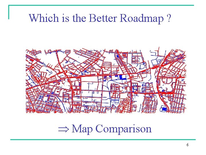
Which is the Better Roadmap ? 5

Which is the Better Roadmap ? Map Comparison 6

Map Construction 7

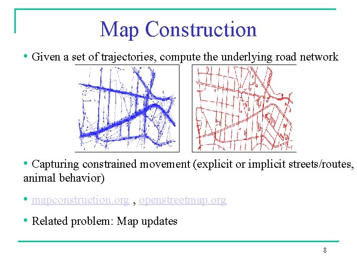
Map Construction • Given a set of trajectories, compute the underlying road network • Capturing constrained movement (explicit or implicit streets/routes, animal behavior) • mapconstruction. org , openstreetmap. org • Related problem: Map updates 8

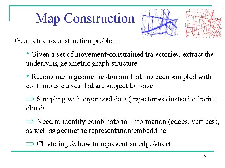
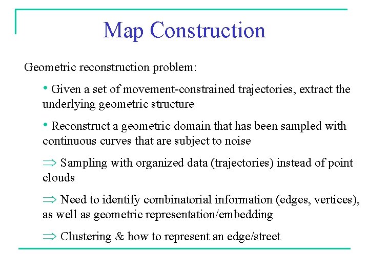
Map Construction Geometric reconstruction problem: • Given a set of movement-constrained trajectories, extract the underlying geometric graph structure • Reconstruct a geometric domain that has been sampled with continuous curves that are subject to noise Sampling with organized data (trajectories) instead of point clouds Need to identify combinatorial information (edges, vertices), as well as geometric representation/embedding Clustering & how to represent an edge/street 9

Input and Output Models Trajectory: A sequence of position samples p 1, …, pn. Each pi minimally consists of a position measurement (e. g. , (x, y)-coordinate) and a time stamp, but may also include other information such as instantaneous speed. Road network: An embedded graph G=(V, E). planar undirected We model the original map and the reconstructed map as embedded undirected graphs in the plane. 10
![Map Construction Approaches BE 12 J Biagioni J Eriksson Map inference in the face Map Construction Approaches [BE 12] J. Biagioni, J. Eriksson, Map inference in the face](https://slidetodoc.com/presentation_image_h2/c8851261d8d36378cd6650fc2cef7703/image-11.jpg)
Map Construction Approaches [BE 12] J. Biagioni, J. Eriksson, Map inference in the face of noise and disparity, 20 th ACM SIGSPATIAL: 79 -88, 2012. [WWL 15] S. Wang, Y. Li , Efficient map reconstruction and augmentation via topological methods. ACM SIGSPATIAL 2015. [DBH 06] J. Davies, A. Beresford, A. Hopper: Scalable, distributed, real-time map generation. IEEE Pervasive Comp. 5(4), 47 -54, 2006. [DWW 18] T. Dey, J. Wang, Y. Wang, Graph Reconstruction by Discrete Morse Theory. Accepted to So. CG 2018.
![Map Construction More Results Topological approach on neighborhood complex GSBW 11 Uses Reeb Map Construction: More Results • Topological approach on neighborhood complex: [GSBW 11]: Uses Reeb](https://slidetodoc.com/presentation_image_h2/c8851261d8d36378cd6650fc2cef7703/image-12.jpg)
Map Construction: More Results • Topological approach on neighborhood complex: [GSBW 11]: Uses Reeb graph to model branching structure [GSBW 11] X. Ge, I. Safa, M. Belkin, Y. Wang, Data skeletonization via Reeb graphs, Conf. Neural Inf. Proc. Systems: 837 -845, 2011.
![Map Construction Even More Results Intersection linking FK 10 KP 12 First detect Map Construction: Even More Results • Intersection linking [FK 10, KP 12]: First detect](https://slidetodoc.com/presentation_image_h2/c8851261d8d36378cd6650fc2cef7703/image-13.jpg)
Map Construction: Even More Results • Intersection linking [FK 10, KP 12]: First detect intersections, then connect them using road segments - [FK 10]: First identify intersections (vertices) using a shape descriptor, then fill in edges. - [KP 12]: Detect intersections from turns and speed change, then fill in edges. • Incremental trajectory insertion [AW 12] • Insert one trajectory at a time. • Use partial Fréchet distance to identify new and existing portions. • Use min-link algorithm to compute representative curve/edge. [AW 12] M. Ahmed, C. Wenk, Constructing Street Networks from GPS Trajectories, ESA: 60 -71, 2012. [FK 10] A. Fathi, J. Krumm, Detecting road intersections from GPS traces, Geographic Information Science, LNCS 6292: 56 -69, 2010. [KP 12] S. Karagiorgou, D. Pfoser, On vehicle-tracking data-based road network generation, 20 th ACM SIGPATIAL: 89 -98, 2012.
![Map Construction AW 12 Incrementally add one trajectory after another For each trajectory 1 Map Construction [AW 12] Incrementally add one trajectory after another. For each trajectory: 1.](https://slidetodoc.com/presentation_image_h2/c8851261d8d36378cd6650fc2cef7703/image-14.jpg)
Map Construction [AW 12] Incrementally add one trajectory after another. For each trajectory: 1. Use partial Fréchet distance to identify new and existing portions by combining mapmatching with partial Fréchet distance: 2. Use min-link curve simplification algorithm to reconcile existing portions [AW 12] M. Ahmed, C. Wenk, Constructing Street Networks from GPS Trajectories, ESA: 60 -71, 2012.

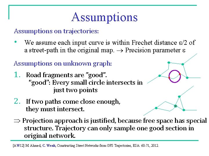
Assumptions on trajectories: • We assume each input curve is within Frechet distance e/2 of a street-path in the original map. Precision parameter e Assumptions on unknown graph: 1. Road fragments are ”good”. “good”: Every small circle intersects in just two points 2. If two paths come close enough, they must intersect. Projection approach is justified, because free space has special structure. Trajectory can only sample one good section in original network. [AW 12] M. Ahmed, C. Wenk, Constructing Street Networks from GPS Trajectories, ESA: 60 -71, 2012.
![Map Construction AW 12 Incrementally add one trajectory after another For each trajectory 1 Map Construction [AW 12] Incrementally add one trajectory after another. For each trajectory: 1.](https://slidetodoc.com/presentation_image_h2/c8851261d8d36378cd6650fc2cef7703/image-16.jpg)
Map Construction [AW 12] Incrementally add one trajectory after another. For each trajectory: 1. Use partial Fréchet distance to identify new and existing portions by combining mapmatching with partial Fréchet distance: 2. Use min-link curve simplification algorithm to reconcile existing portions [AW 12] M. Ahmed, C. Wenk, Constructing Street Networks from GPS Trajectories, ESA: 60 -71, 2012.

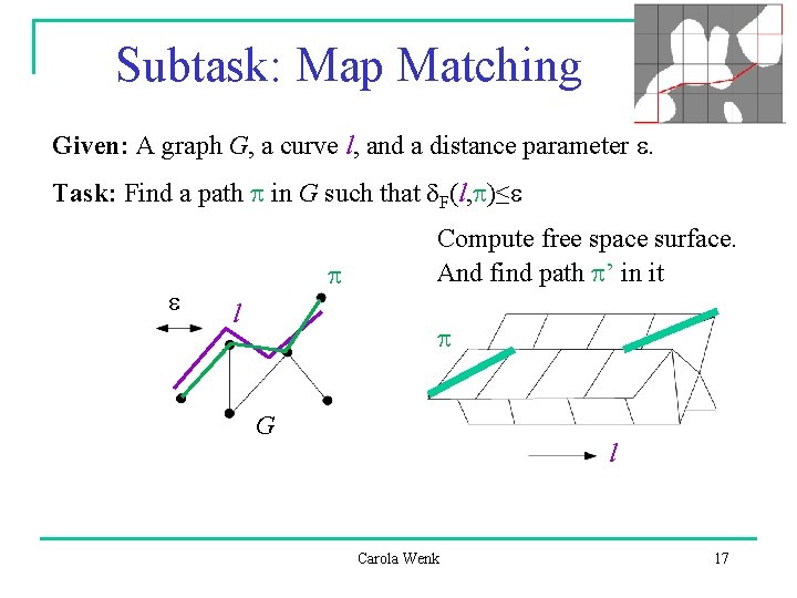
Subtask: Map Matching Given: A graph G, a curve l, and a distance parameter e. Task: Find a path p in G such that d. F(l, p)≤e e p l Compute free space surface. And find path p’ in it p G l Carola Wenk 17

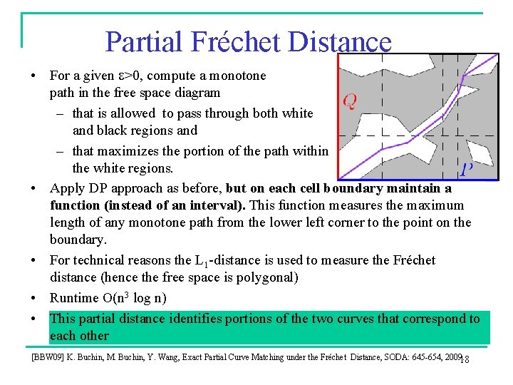
Partial Fréchet Distance • For a given e>0, compute a monotone path in the free space diagram – that is allowed to pass through both white and black regions and – that maximizes the portion of the path within the white regions. • Apply DP approach as before, but on each cell boundary maintain a function (instead of an interval). This function measures the maximum length of any monotone path from the lower left corner to the point on the boundary. • For technical reasons the L 1 -distance is used to measure the Fréchet distance (hence the free space is polygonal) • Runtime O(n 3 log n) • This partial distance identifies portions of the two curves that correspond to each other [BBW 09] K. Buchin, M. Buchin, Y. Wang, Exact Partial Curve Matching under the Fréchet Distance, SODA: 645 -654, 2009. 18
![Map Construction AW 12 Incrementally add one trajectory after another For each trajectory 1 Map Construction [AW 12] Incrementally add one trajectory after another. For each trajectory: 1.](https://slidetodoc.com/presentation_image_h2/c8851261d8d36378cd6650fc2cef7703/image-19.jpg)
Map Construction [AW 12] Incrementally add one trajectory after another. For each trajectory: 1. Use partial Fréchet distance to identify new and existing portions by combining mapmatching with partial Fréchet distance: • Compute free space surface • Find path that maximizes matched portion on the curve. Project free space onto curve: white interval = matched portion, black interval = unmatched portion 2. Use min-link curve simplification algorithm to reconcile existing portions [AW 12] M. Ahmed, C. Wenk, Constructing Street Networks from GPS Trajectories, ESA: 60 -71, 2012.

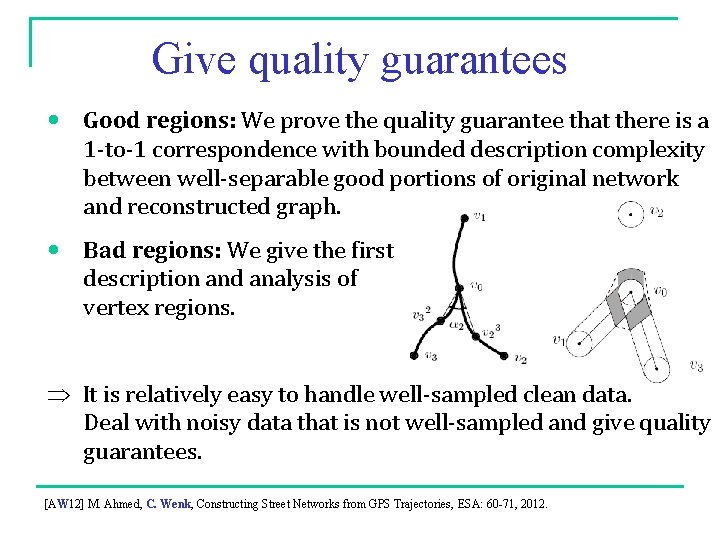
Give quality guarantees • Good regions: We prove the quality guarantee that there is a 1 -to-1 correspondence with bounded description complexity between well-separable good portions of original network and reconstructed graph. • Bad regions: We give the first description and analysis of vertex regions. It is relatively easy to handle well-sampled clean data. Deal with noisy data that is not well-sampled and give quality guarantees. [AW 12] M. Ahmed, C. Wenk, Constructing Street Networks from GPS Trajectories, ESA: 60 -71, 2012.
![Map Construction AW 12 Incrementally add one trajectory after another For each trajectory 1 Map Construction [AW 12] Incrementally add one trajectory after another. For each trajectory: 1.](https://slidetodoc.com/presentation_image_h2/c8851261d8d36378cd6650fc2cef7703/image-21.jpg)
Map Construction [AW 12] Incrementally add one trajectory after another. For each trajectory: 1. Use partial Fréchet distance to identify new and existing portions by combining mapmatching with partial Fréchet distance: • Compute free space surface • Find path that maximizes matched portion on the curve. Project free space onto curve: white interval = matched portion, black interval = unmatched portion 2. Use min-link curve simplification algorithm to reconcile existing portions [AW 12] M. Ahmed, C. Wenk, Constructing Street Networks from GPS Trajectories, ESA: 60 -71, 2012.

Curve Simplification • Arbitrary vertices: • min-#: Compute a minimum link path that stabs e-neighborhoods around vertices of f in the correct order. O(n) time. • min-e: Binary search on critical values. O(n 2) time. • Subsequence of original vertices: • Douglas-Peucker algorithm, O(n log n) time. • min-#: Add shortcut-edges between vertices if shortcut is within error e. Then find a path with min-# edges. O(n 2) time, and O(n 4/3+d) for x-monotone chains. [AG 99] H. Alt, L. Guibas, Discrete Geometric Shapes…, Handbook of Computational Geometry: 121 -153, 1999. [GHMS 93] L. Guibas, J. Hershberger, J. Mitchell, J. Snoeyink, Approximating …, minimum link paths, IJCGA 3(4): 383 -415, 1993 [II 88] H. Imai, M. Iri, Polygonal approximations of a curve…, in Computational Morphology, Toussaint (eds): 71 -86, 1988

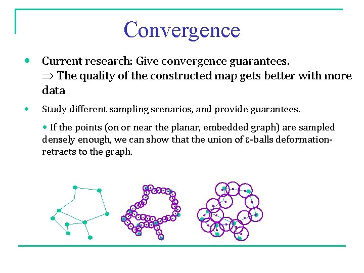
Convergence • Current research: Give convergence guarantees. The quality of the constructed map gets better with more data • Study different sampling scenarios, and provide guarantees. • If the points (on or near the planar, embedded graph) are sampled densely enough, we can show that the union of e-balls deformationretracts to the graph.

Different Reconstructions GPS Trajectory Data Reconstructed Maps 24

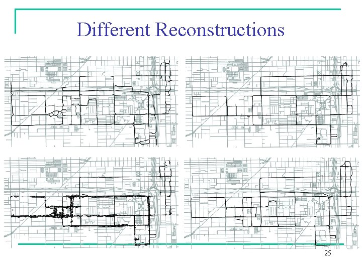
Different Reconstructions 25

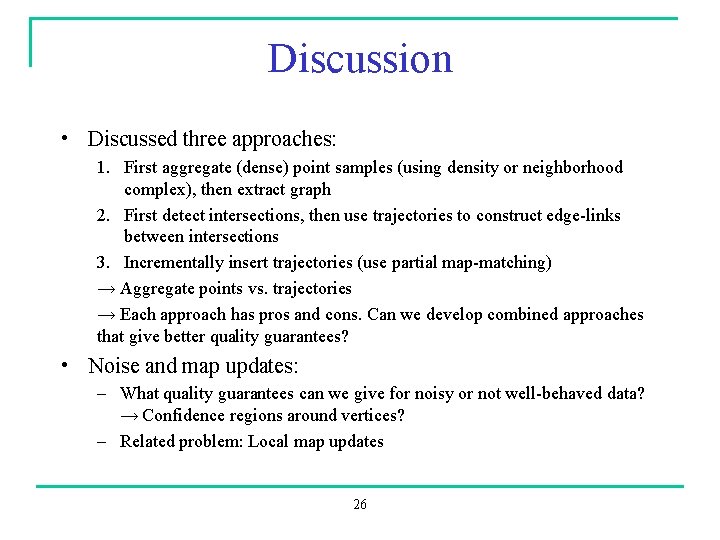
Discussion • Discussed three approaches: 1. First aggregate (dense) point samples (using density or neighborhood complex), then extract graph 2. First detect intersections, then use trajectories to construct edge-links between intersections 3. Incrementally insert trajectories (use partial map-matching) → Aggregate points vs. trajectories → Each approach has pros and cons. Can we develop combined approaches that give better quality guarantees? • Noise and map updates: – What quality guarantees can we give for noisy or not well-behaved data? → Confidence regions around vertices? – Related problem: Local map updates 26


Reconciling Trajectory Sets

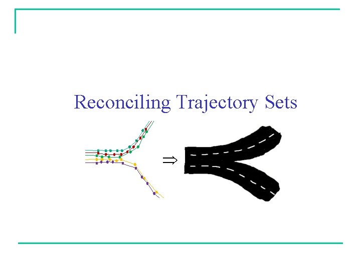
Reconciling Trajectory Sets Given a set of trajectories Compute an average/mean or median trajectory Ø Reconcile the set into one representative trajectory Ø Prerequisite for k-means and k-medoid clustering Ø Related: Curve Simplification (reduce complexity) Compute (sub-)trajectory clusters Ø Find similar parts of the trajectories Ø For each cluster, compute a reconciled representation Compute a road network Ø Find a graph structure representing all trajectories

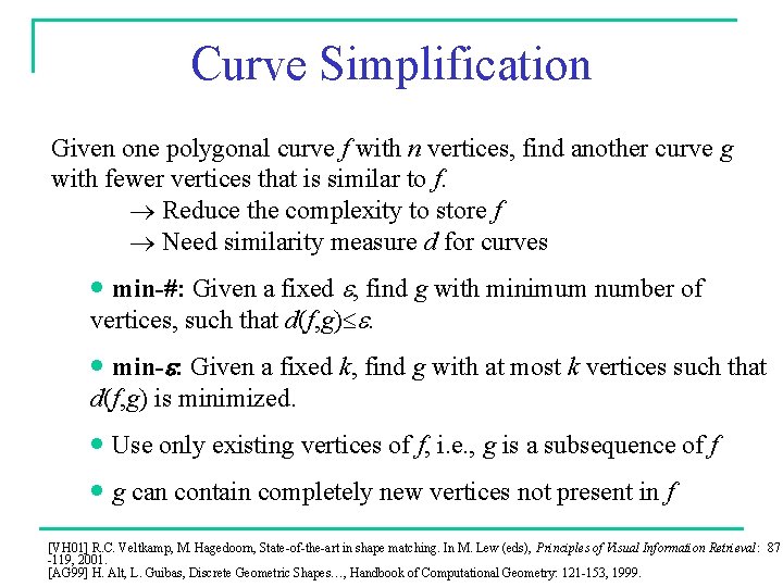
Curve Simplification Given one polygonal curve f with n vertices, find another curve g with fewer vertices that is similar to f. Reduce the complexity to store f Need similarity measure d for curves min-#: Given a fixed e, find g with minimum number of vertices, such that d(f, g) e. min-e: Given a fixed k, find g with at most k vertices such that d(f, g) is minimized. Use only existing vertices of f, i. e. , g is a subsequence of f g can contain completely new vertices not present in f [VH 01] R. C. Veltkamp, M. Hagedoorn, State-of-the-art in shape matching. In M. Lew (eds), Principles of Visual Information Retrieval: 87 -119, 2001. [AG 99] H. Alt, L. Guibas, Discrete Geometric Shapes…, Handbook of Computational Geometry: 121 -153, 1999.

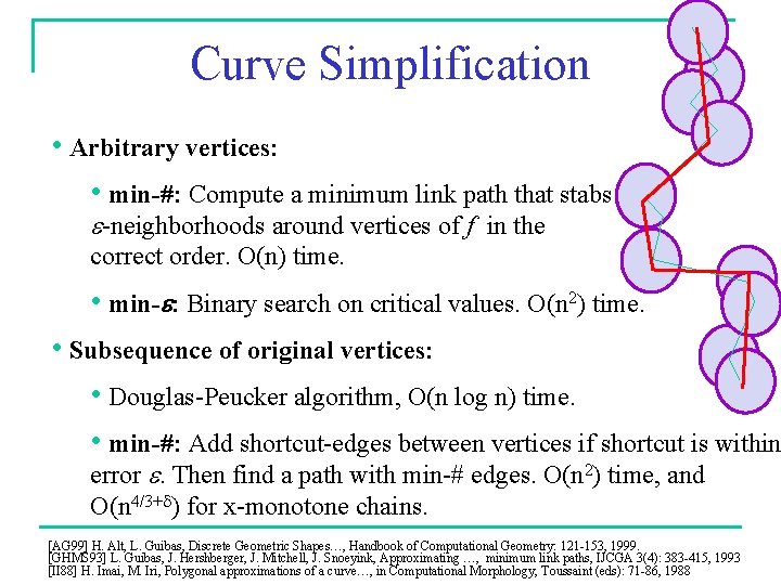
Curve Simplification • Arbitrary vertices: • min-#: Compute a minimum link path that stabs e-neighborhoods around vertices of f in the correct order. O(n) time. • min-e: Binary search on critical values. O(n 2) time. • Subsequence of original vertices: • Douglas-Peucker algorithm, O(n log n) time. • min-#: Add shortcut-edges between vertices if shortcut is within error e. Then find a path with min-# edges. O(n 2) time, and O(n 4/3+d) for x-monotone chains. [AG 99] H. Alt, L. Guibas, Discrete Geometric Shapes…, Handbook of Computational Geometry: 121 -153, 1999. [GHMS 93] L. Guibas, J. Hershberger, J. Mitchell, J. Snoeyink, Approximating …, minimum link paths, IJCGA 3(4): 383 -415, 1993 [II 88] H. Imai, M. Iri, Polygonal approximations of a curve…, in Computational Morphology, Toussaint (eds): 71 -86, 1988

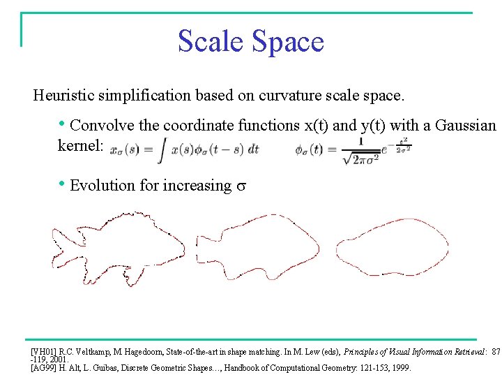
Scale Space Heuristic simplification based on curvature scale space. • Convolve the coordinate functions x(t) and y(t) with a Gaussian kernel: • Evolution for increasing s [VH 01] R. C. Veltkamp, M. Hagedoorn, State-of-the-art in shape matching. In M. Lew (eds), Principles of Visual Information Retrieval: 87 -119, 2001. [AG 99] H. Alt, L. Guibas, Discrete Geometric Shapes…, Handbook of Computational Geometry: 121 -153, 1999.
![AverageMean Curve Given a set f 1 fk 0 1 R 2 Average/Mean Curve Given a set f 1, …, fk : [0, 1] R 2](https://slidetodoc.com/presentation_image_h2/c8851261d8d36378cd6650fc2cef7703/image-33.jpg)
Average/Mean Curve Given a set f 1, …, fk : [0, 1] R 2 of trajectories/curves, compute one reconciled curve that represents all curves in the set: • Point-wise average: f(t) = 1/n n i=1 fi for all t [0, 1]. O(kn) time. But only works if parameterizations of curves correspond to each other! • Compute k-dimensional free space (use concept of Fréchet distance for sets of curves). Instead of Euclidean distance use the radius of the minimum enclosing disk for k points. O(nk) time. Tries out all joint reparameterizations of curves. [DR 04] A. Dumitrescu, G. Rote, On the Fréchet Distance of a Set of Curves, CCCG: 162 -165, 2004. [HR 11] S. Har-Peled, B. Raichel, The Fréchet Distance Revisited and Extended, ACM So. CG: 448 -457, 2011.

Average vs. Median The average is allowed to introduce new vertices and curve pieces. Can one compute a median, which uses only existing curve pieces and which is central with respect to number of trajectories? • E. g. , 2 hiking trajectories on one side of lake, 3 on other side of lake. Average trajectory would go through lake. • Median of k numbers is the k/2 -smallest number. • k/2 -level in arrangement of lines (has O(k 4/3) complexity): [BBKLSWW 12] K. & M. Buchin, M. van Kreveld, M. Löffler, R. Silveira, C. Wenk, L. Wiratma, Median Trajectories, Algorithmica, Online First, 2012.

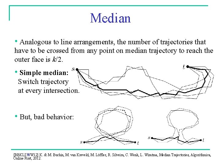
Median • Analogous to line arrangements, the number of trajectories that have to be crossed from any point on median trajectory to reach the outer face is k/2. • Simple median: Switch trajectory at every intersection. • But, bad behavior: [BBKLSWW 12] K. & M. Buchin, M. van Kreveld, M. Löffler, R. Silveira, C. Wenk, L. Wiratma, Median Trajectories, Algorithmica, Online First, 2012.

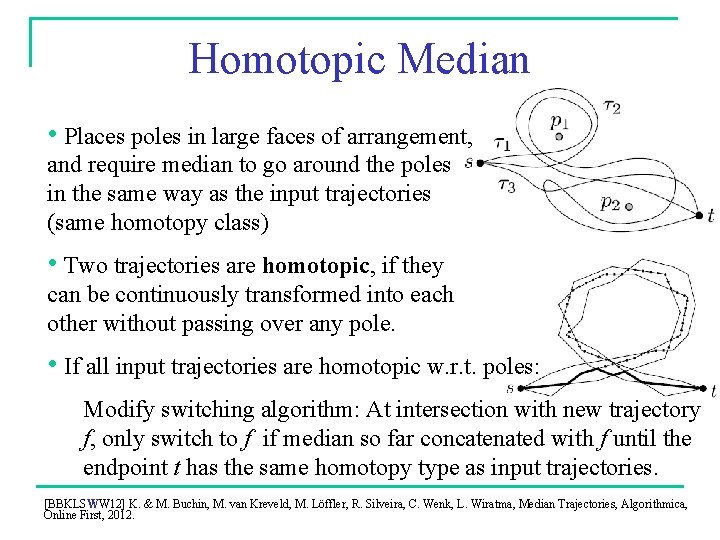
Homotopic Median • Places poles in large faces of arrangement, and require median to go around the poles in the same way as the input trajectories (same homotopy class) • Two trajectories are homotopic, if they can be continuously transformed into each other without passing over any pole. • If all input trajectories are homotopic w. r. t. poles: Modify switching algorithm: At intersection with new trajectory f, only switch to f if median so far concatenated with f until the endpoint t has the same homotopy type as input trajectories. [BBKLSWW 12] K. & M. Buchin, M. van Kreveld, M. Löffler, R. Silveira, C. Wenk, L. Wiratma, Median Trajectories, Algorithmica, Online First, 2012.

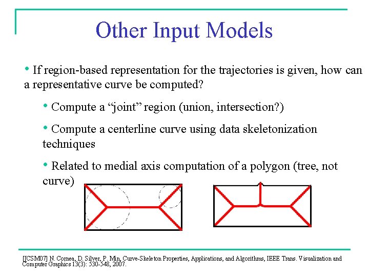
Other Input Models • If region-based representation for the trajectories is given, how can a representative curve be computed? • Compute a “joint” region (union, intersection? ) • Compute a centerline curve using data skeletonization techniques • Related to medial axis computation of a polygon (tree, not curve) [[CSM 07] N. Cornea, D. Silver, P. Min, Curve-Skeleton Properties, Applications, and Algorithms, IEEE Trans. Visualization and Computer Graphics 13(3): 530 -548, 2007.

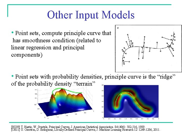
Other Input Models • Point sets, compute principle curve that has smoothness condition (related to linear regression and principal components) • Point sets with probability densities, principle curve is the “ridge” of the probability density “terrain” [HS 89] T. Hastie, W. Stuetzle, Principal Curves, J. American Statistical Association 84 (406): 502 -516, 1989. [OE 11] U. Ozertem, D. Erdogmus, Locally Defined Principal Curves, J. Machine Learning Research 12: 1249 -1286, 2011.

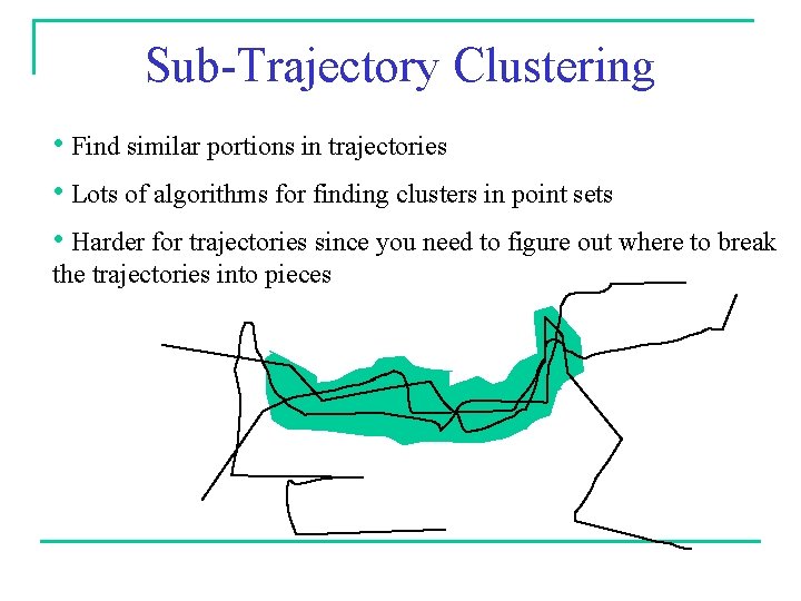
Sub-Trajectory Clustering • Find similar portions in trajectories • Lots of algorithms for finding clusters in point sets • Harder for trajectories since you need to figure out where to break the trajectories into pieces

Sub-Trajectory Clustering • A. Asahara, A. Sato, and K. Maruyama. Evaluation of trajectory clustering based on information criteria for human activity analysis. In 10 th Int. Conf. on Mobile Data Management: Systems, Services and Middleware (MDM), pages 329 -337, 2009. • K. Buchin, M. Buchin, J. Gudmundsson, M. L öffler, and J. Luo. Detecting commuting patterns by clustering subtrajectories. International Journal of Computational Geometry and Applications, special issue on 19 th International Symposium on Algorithms and Computation (ISAAC), 2010. • K. Buchin, M. van Kreveld, and J. Luo. Finding long and similar parts of trajectories. In 17 th ACM SIGSPATIAL International Conference on Advances in Geographic Information Systems (ACM GIS), pages 296 -305, 2010. • A. Dahlbom and L. Niklasson. Trajectory clustering for coastal surveillance. In 10 th Int. Conf. on Information Fusion, pages 1 -8, 2007. • J. Lee, J. Han, and K. -Y. Whang. Trajectory clustering: A partition-and-group framework. In Proc. ACM SIGMOD International Conference on Management of Data, pages 593 -604, 2007.

Sub-Trajectory Clustering • X. Li, W. Hu, and W. Hu. A coarse-to-ne strategy for vehicle motion trajectory clustering. In 18 th Int. Conf. on Pattern Recognition (ICPR), volume 1, pages 591 -594, 2006. • Z. Li. Incremental clustering for trajectories. Master's thesis, University of Illinois at Urbana-Champaign, 2010. • Z. Li, J. -G. Lee, X. Li, and J. Han. Incremental clustering for trajectories. In Proc. 15 th Int. Conf. Database Systems for Advanced Applications (DASFAA), pages 32 -46, 2010. • T. W. Liao. Clustering of time series data - a survey. Pattern Recognition, 38: 1857 -1874, 2005. • Y. Zhang and D. Pi. A trajectory clustering algorithm based on symmetric neighborhood. In WRI World Congrees on Computer Science and Information Engineering, volume 3, pages 640 -645, 2009.

Fréchet-Based Clustering • Given an input set of trajectories, append them all to form a single trajectory f • Compute the free space diagram of f with itself (comparing f with f) • Find clusters of monotone curve pieces in the (white) free space Sweep free space from left to right, maintain data structure [BBGLL 10] K. Buchin, M. Buchin, J. Gudmundsson, M. Löffler, J. Luo. Detecting commuting patterns…, IJCGA, 2010.

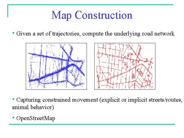
Map Construction • Given a set of trajectories, compute the underlying road network • Capturing constrained movement (explicit or implicit streets/routes, animal behavior) • Open. Street. Map

Map Construction Geometric reconstruction problem: • Given a set of movement-constrained trajectories, extract the underlying geometric structure • Reconstruct a geometric domain that has been sampled with continuous curves that are subject to noise Sampling with organized data (trajectories) instead of point clouds Need to identify combinatorial information (edges, vertices), as well as geometric representation/embedding Clustering & how to represent an edge/street
![Some Results CGHS 10 First algorithm with quality guarantees Subsamples trajectories Dense point Some Results • [CGHS 10]: First algorithm with quality guarantees. Subsamples trajectories Dense point](https://slidetodoc.com/presentation_image_h2/c8851261d8d36378cd6650fc2cef7703/image-45.jpg)
Some Results • [CGHS 10]: First algorithm with quality guarantees. Subsamples trajectories Dense point cloud. Uses local neighborhood simplicial complexes. Reconstructs “good” portions of edges. • [ACCGGM 11]: Reconstruct “metric graph” from point cloud. Compute almost isometric space with lower complexity. Focuses on combinatorial information and not on embedding. Quality guarantees assume dense sampling. • [GSBW 11]: Topological approach on neighborhood complex. Uses Reeb graph to model skeleton graph (branching structure) [ACCGGM 11] M. Aanjaneya, F. Chazal, D. Chen, M. Glisse, L. Guibas, D. Morozov. Metric graph reconstruction…, So. CG, 2011. [CGHS 10] D. Chen, L. Guibas, J. Hershberger, J. Sun, Road network reconstruction for organizing paths, SODA, 2010. [GSBW 11] X. Ge, I. Safa, M. Belkin, Y. Wang, Data skeletonization via Reeb graphs, Conf. Neural Inf. Proc. Systems: 837 -845, 2011.
![Some More Results FK 10 First identify intersections vertices using a shape descriptor Some More Results • [FK 10]: First identify intersections (vertices) using a shape descriptor,](https://slidetodoc.com/presentation_image_h2/c8851261d8d36378cd6650fc2cef7703/image-46.jpg)
Some More Results • [FK 10]: First identify intersections (vertices) using a shape descriptor, then fill in edges. • [AW 12]: Use trajectory information. Incrementally add one trajectory after another. Use partial Fréchet distance to identify new and existing portions. Use min-link algorithm to compute representative curve/edge. [FK 10] A. Fathi, J. Krumm, Detecting road intersections from GPS traces, Geographic Information Science, LNCS 6292: 56 -69, 2010. [AW 12] M. Ahmed, C. Wenk, Constructing Street Networks from GPS Trajectories, ESA, to appear, 2012.
![CGHS 10 Algorithm Steps 1 2 3 4 5 Compute benet subsample to obtain [CGHS 10] Algorithm Steps 1. 2. 3. 4. 5. Compute be-net (subsample to obtain](https://slidetodoc.com/presentation_image_h2/c8851261d8d36378cd6650fc2cef7703/image-47.jpg)
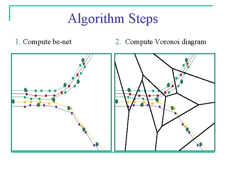
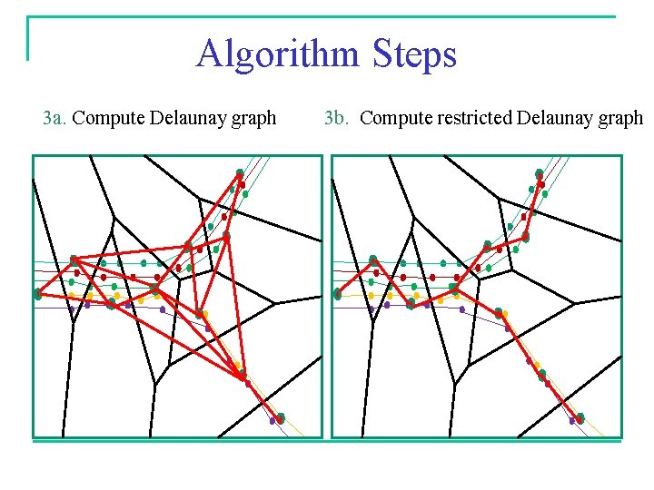
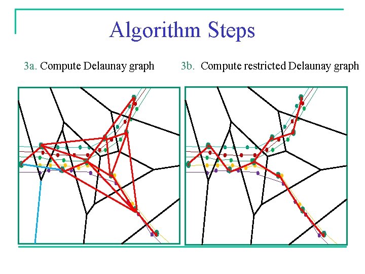
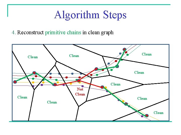
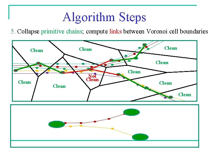
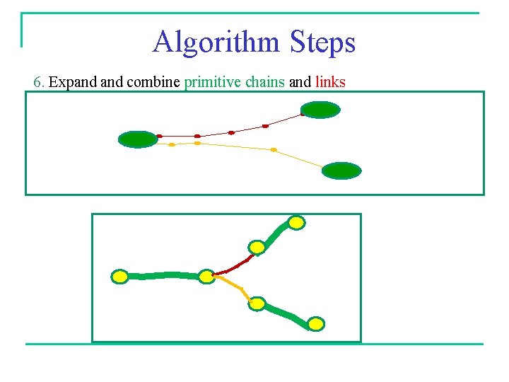
[CGHS 10] Algorithm Steps 1. 2. 3. 4. 5. Compute be-net (subsample to obtain point cloud) Compute Voronoi diagram for point cloud Compute clean, restricted Delaunay graph Reconstruct primitive chains Collapse primitive chains; compute links between Voronoi cell boundaries 6. Expand combine primitive chains and links

Algorithm Steps 1. Compute be-net 2. Compute Voronoi diagram

Algorithm Steps 3 a. Compute Delaunay graph 3 b. Compute restricted Delaunay graph

Algorithm Steps 3 a. Compute Delaunay graph 3 b. Compute restricted Delaunay graph

Algorithm Steps 3 c. Compute graph between “clean” Voronoi cells: degree 2 there is an input path cutting “properly” through cell Clean Clean Not Clean Clean

Algorithm Steps 4. Reconstruct primitive chains in clean graph Clean Clean Not Clean Clean

Algorithm Steps 5. Collapse primitive chains; compute links between Voronoi cell boundaries Clean Clean Not Clean Clean

Algorithm Steps 6. Expand combine primitive chains and links

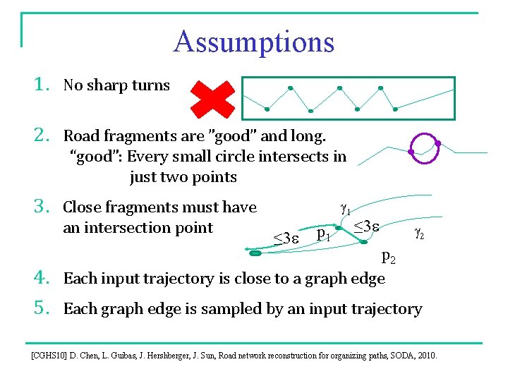
Assumptions 1. No sharp turns 2. Road fragments are ”good” and long. “good”: Every small circle intersects in just two points 3. Close fragments must have an intersection point g 1 ≤ 3 e p 1 ≤ 3 e g 2 p 2 Each input trajectory is close to a graph edge 4. 5. Each graph edge is sampled by an input trajectory [CGHS 10] D. Chen, L. Guibas, J. Hershberger, J. Sun, Road network reconstruction for organizing paths, SODA, 2010.

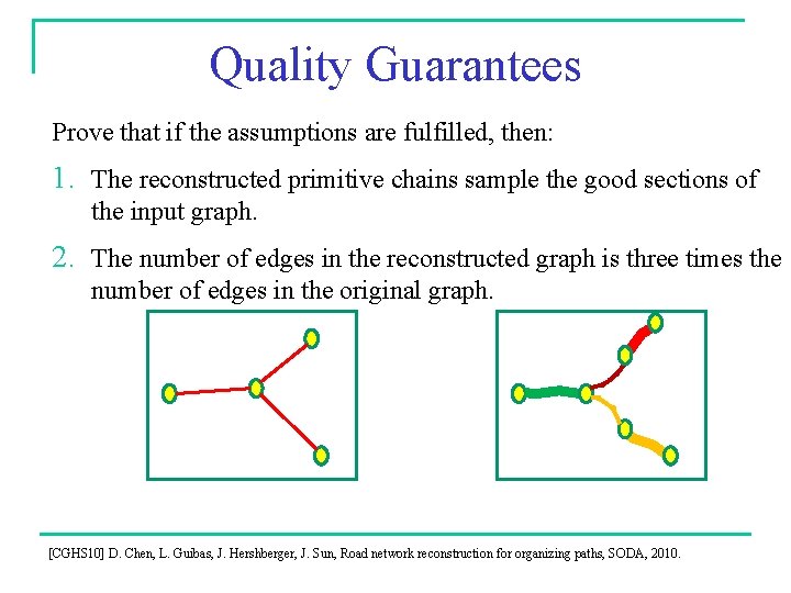
Quality Guarantees Prove that if the assumptions are fulfilled, then: 1. The reconstructed primitive chains sample the good sections of the input graph. 2. The number of edges in the reconstructed graph is three times the number of edges in the original graph. [CGHS 10] D. Chen, L. Guibas, J. Hershberger, J. Sun, Road network reconstruction for organizing paths, SODA, 2010.
![AW 12 Incrementally add one trajectory after another For each trajectory 1 Use partial [AW 12] Incrementally add one trajectory after another. For each trajectory: 1. Use partial](https://slidetodoc.com/presentation_image_h2/c8851261d8d36378cd6650fc2cef7703/image-57.jpg)
[AW 12] Incrementally add one trajectory after another. For each trajectory: 1. Use partial Fréchet distance to identify new and existing portions by combining mapmatching with partial Fréchet distance: • Compute free space surface (à la map-matching) • Find path that minimizes black portions, but measure path length only along the curve (not along graph) Project free space onto curve, yielding sequence of intervals which is easy to process. 2. Use min-link algorithm to reconcile existing portions [AW 12] M. Ahmed, C. Wenk, Constructing Street Networks from GPS Trajectories, ESA, to appear, 2012.

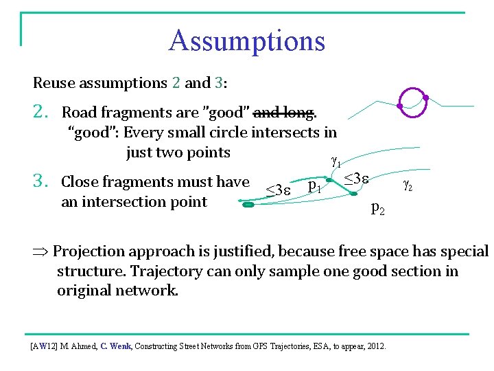
Assumptions Reuse assumptions 2 and 3: 2. Road fragments are ”good” and long. “good”: Every small circle intersects in just two points g 3. Close fragments must have ≤ 3 e p 1 an intersection point 1 ≤ 3 e g 2 p 2 Projection approach is justified, because free space has special structure. Trajectory can only sample one good section in original network. [AW 12] M. Ahmed, C. Wenk, Constructing Street Networks from GPS Trajectories, ESA, to appear, 2012.

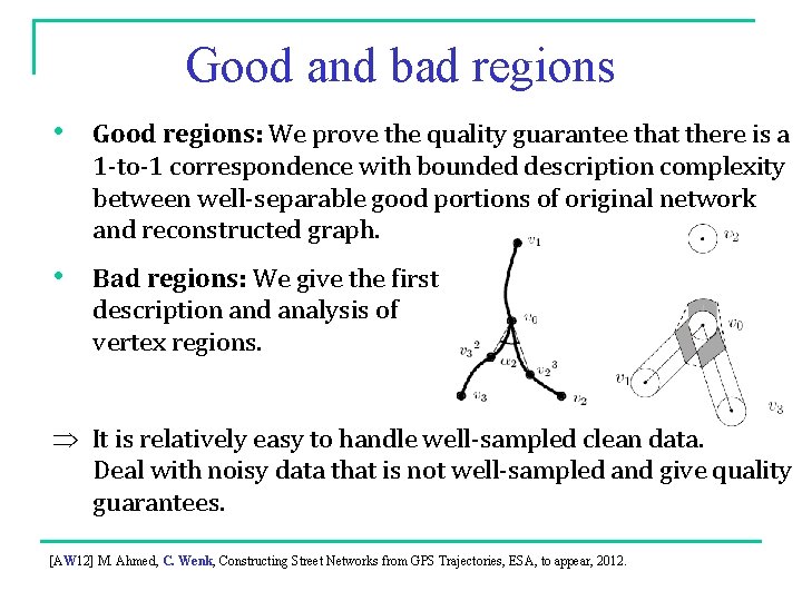
Good and bad regions • Good regions: We prove the quality guarantee that there is a 1 -to-1 correspondence with bounded description complexity between well-separable good portions of original network and reconstructed graph. • Bad regions: We give the first description and analysis of vertex regions. It is relatively easy to handle well-sampled clean data. Deal with noisy data that is not well-sampled and give quality guarantees. [AW 12] M. Ahmed, C. Wenk, Constructing Street Networks from GPS Trajectories, ESA, to appear, 2012.

Discussion • Develop uncertainty models for the input (= trajectories) and the output. Develop algorithms (reconciling, map construction, etc. ) for these models. • Dual problem, keep trajectories for each road segment • Use information from usual routes that people take Find combination of trajectories to route. Use results of previous queries/views to compute routing.