Algorithms for Big Data Streaming and Sublinear Time
Algorithms for Big Data: Streaming and Sublinear Time Algorithms Moran Feldman
Motivation Big Data (huge data sets) Why? So What? • The Internet q Easy to collect data q Easy to transfer data • New equipment q LHC • Difficult to process all the data. • Difficult to store all the data. 2
What is this Talk About? • Big data has motivated a lot of research (both CS and non-CS). • In this talk we are interested in theoretical algorithms for big data problems. – Sublinear time algorithms – Streaming Algorithms • We will see a few classical algorithms of each one of these kinds. 3
Sublinear Time Algorithms
Sublinear Time Algorithms • Most algorithms read all their input. – Require at least a linear time. • We are interested in sublinear time algorithms. – Cannot afford to read all its input. • We will start with a simple example… 5
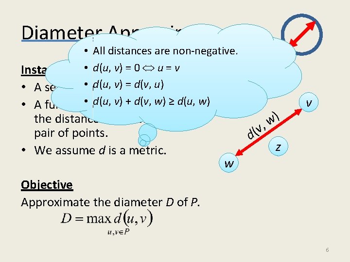
Diameter Approximation • All distances are non-negative. Instance • d(u, v) = 0 u = v u d(u, v) = d(v, u) • A set P of • points. d(u, + d(v, ≥ d(u, w) • A function • d: P v) P Rw)giving the distance between every pair of points. • We assume d is a metric. v ( d w ) w , v z Objective Approximate the diameter D of P. 6
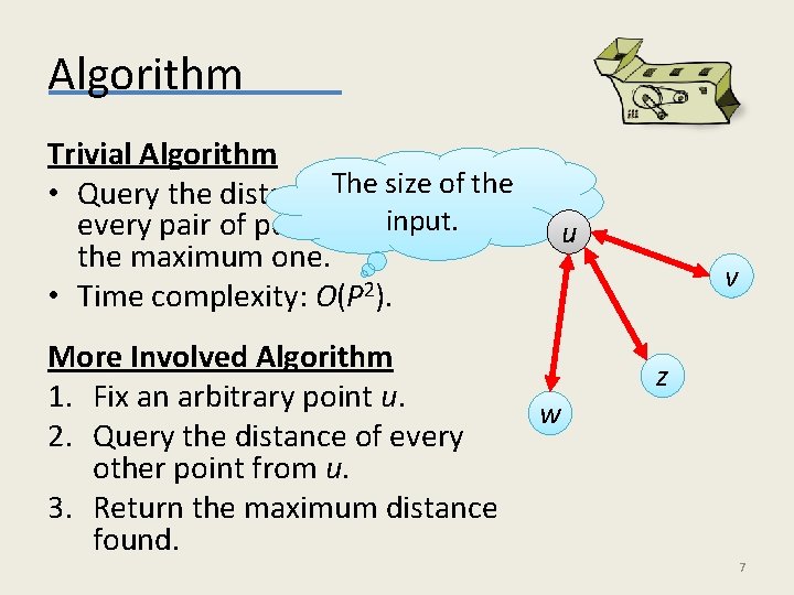
Algorithm Trivial Algorithm size of the • Query the distance. The between input. every pair of points, and return the maximum one. • Time complexity: O(P 2). More Involved Algorithm 1. Fix an arbitrary point u. 2. Query the distance of every other point from u. 3. Return the maximum distance found. u v w z 7
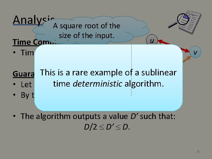
Analysis. A square root of the size of the input. Time Complexity • Time O(P). u v This is a rare example of a sublinear Guarantee z time deterministic • Let d(v, w) be the diameter. algorithm. w • By the triangle inequality: d(u, v) + d(u, w) d(v, w) = D. • The algorithm outputs a value D’ such that: D/2 D’ D. 8
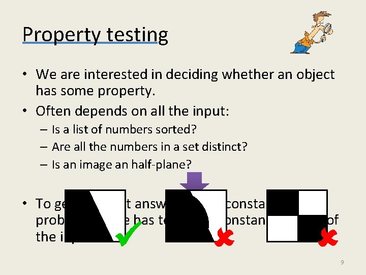
Property testing • We are interested in deciding whether an object has some property. • Often depends on all the input: – Is a list of numbers sorted? – Are all the numbers in a set distinct? – Is an image an half-plane? • To get the right answer with a constant probability one has to read a constant fraction of the input. 9
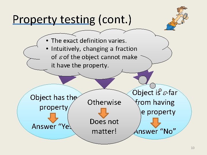
Property testing (cont. ) • The exact definition varies. Distinguish • Intuitively, changing a fraction between two cases of the object cannot make it have the property. Object has the property Otherwise Answer “Yes” Does not matter! Object is -far from having the property Answer “No” 10
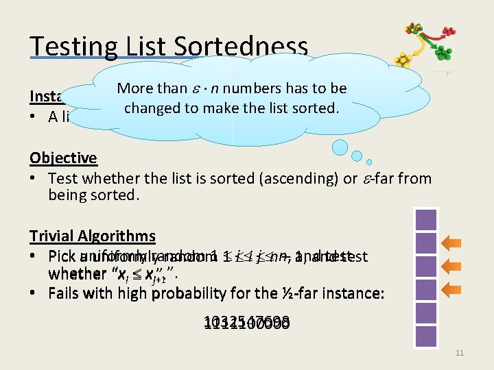
Testing List Sortedness More than n numbers has to be Instance changed to make the list sorted. • A list of numbers of n numbers. Objective • Test whether the list is sorted (ascending) or -far from being sorted. Trivial Algorithms • Pick uniformly and test a uniformlyrandom 1 1 i i j nn, – 1, and test whether “xi xji+1 ”. ”. • Fails with high probability for the ½-far instance: 1032547698 1111100000 11
![Algorithm [EKKRV 00] 1. Pick a uniformly random i. 2. Run a binary search Algorithm [EKKRV 00] 1. Pick a uniformly random i. 2. Run a binary search](http://slidetodoc.com/presentation_image_h/0810b03c1a064a6387366b6605b31b93/image-12.jpg)
Algorithm [EKKRV 00] 1. Pick a uniformly random i. 2. Run a binary search for xi. 3. Answer “No” if the binary search ends up at a point other than i (and “Yes” otherwise). x 4 x 2 x 1 x 6 x 3 x 5 x 7 12
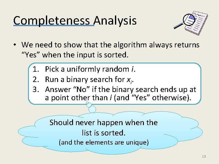
Completeness Analysis • We need to show that the algorithm always returns “Yes” when the input is sorted. 1. Pick a uniformly random i. 2. Run a binary search for xi. 3. Answer “No” if the binary search ends up at a point other than i (and “Yes” otherwise). Should never happen when the list is sorted. (and the elements are unique) 13
Soundness Analysis • We need to upper bound the probability that the algorithm returns “Yes” when the list is -far from being sorted. • An index i is “good” if the algorithm returns “Yes” when it randomly chooses i. • Clearly: Number of Good Indexes Probability n of “Yes” = • Thus, we want to upper bound the number of good idexes in an -far list. 14
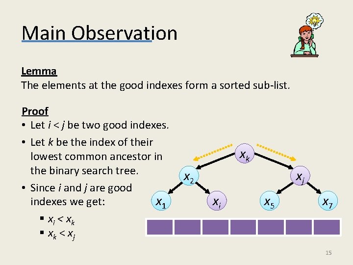
Main Observation Lemma The elements at the good indexes form a sorted sub-list. Proof • Let i < j be two good indexes. • Let k be the index of their lowest common ancestor in the binary search tree. • Since i and j are good x 1 indexes we get: § xi < x k § xk < xj x 4 k x 2 x 6 j x 3 i x 5 x 7 15
Soundness Analysis (cont. ) In an -far list: • No (1 - )n elements can form a sorted sub-list. • There are less than (1 - )n good elements. The algorithm answers “Yes” with probability less than: 1 - • Can be improved by repetition. failsyields with high • Repeating the algorithm. Never -1 times an algorithm that: a ½-far input. – Always answer “Yes”probability for a sorted for input. – Answer “No” for an -far input with probability at least 1/e 0. 367. • Time complexity: O( -1 log n) 16
Streaming Algorithms
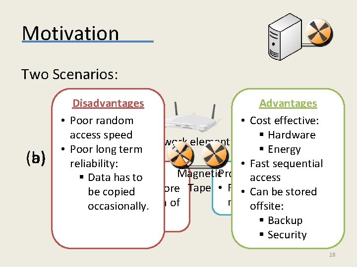
Motivation Two Scenarios: (b) (a) Disadvantages Advantages Network • Poor random • Cost effective: traffic access speed § Hardware A network element • Poor long term § Energy reliability: • Fast sequential the traffic: Magnetic. Processes Problem § Data has to access detects The be element copiedcan store Tape • For • example, Can be stored malicious activity. onlyoccasionally. a small fraction of offsite: the traffic. § Backup § Security 18
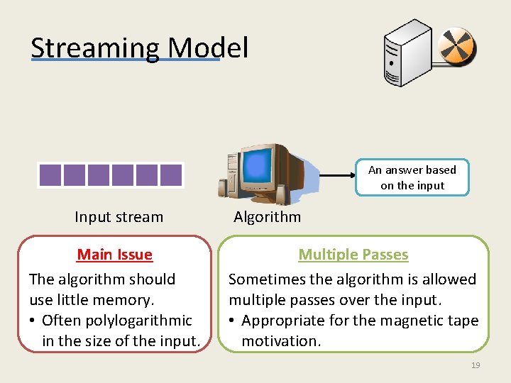
Streaming Model An answer based on the input Input stream Main Issue The algorithm should use little memory. • Often polylogarithmic in the size of the input. Algorithm Multiple Passes Sometimes the algorithm is allowed multiple passes over the input. • Appropriate for the magnetic tape motivation. 19
![Finding Frequent Elements Theorem [MG 82] There is a streaming algorithm using O(k (log Finding Frequent Elements Theorem [MG 82] There is a streaming algorithm using O(k (log](http://slidetodoc.com/presentation_image_h/0810b03c1a064a6387366b6605b31b93/image-20.jpg)
Finding Frequent Elements Theorem [MG 82] There is a streaming algorithm using O(k (log n + log m)) space which: • Outputs a set of at most k – 1 elements. • The set contains every element with more than n/k appearances in the stream. Remarks • A second pass can be used to detect the elements that really have more than n/k appearances. • For simplicity, we present the algorithm for the case k = 2. • Occasionally comes up in job interviews. 20
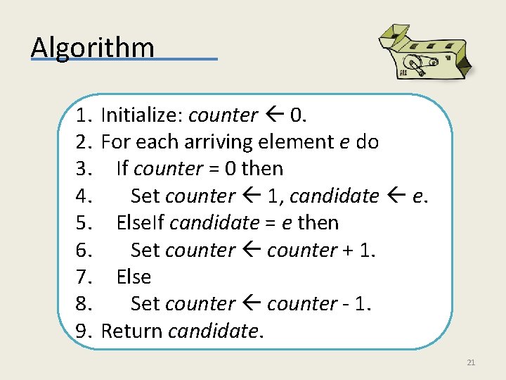
Algorithm 1. Initialize: counter 0. 2. For each arriving element e do 3. If counter = 0 then 4. Set counter 1, candidate e. 5. Else. If candidate = e then 6. Set counter + 1. 7. Else 8. Set counter - 1. 9. Return candidate. 21
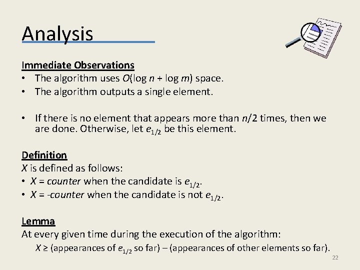
Analysis Immediate Observations • The algorithm uses O(log n + log m) space. • The algorithm outputs a single element. • If there is no element that appears more than n/2 times, then we are done. Otherwise, let e 1/2 be this element. Definition X is defined as follows: • X = counter when the candidate is e 1/2. • X = -counter when the candidate is not e 1/2. Lemma At every given time during the execution of the algorithm: X ≥ (appearances of e 1/2 so far) – (appearances of other elements so far). 22
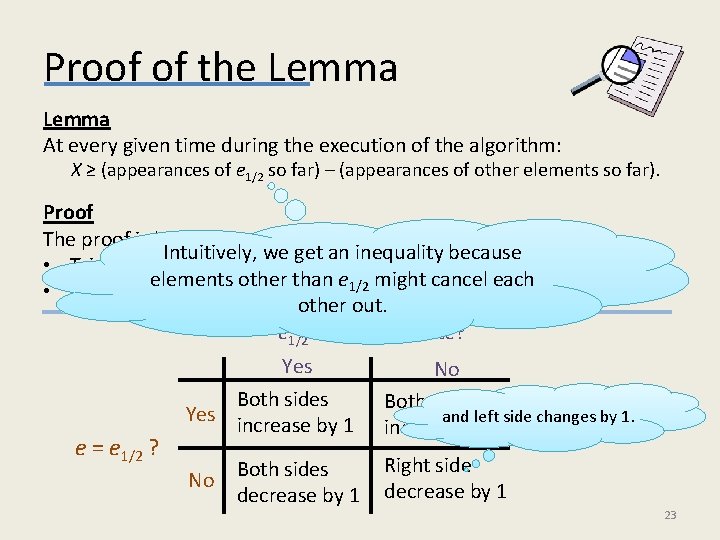
Proof of the Lemma At every given time during the execution of the algorithm: X ≥ (appearances of e 1/2 so far) – (appearances of other elements so far). Proof The proof is by induction. Intuitively, we get an inequality because • Trivially holds before the first element arrives. elements other than e 1/2 might cancel each • Assume it holds before the arrival of an element e, then: other out. e 1/2 is the candidate? e = e 1/2 ? Yes Both sides Yes increase by 1 No Both sides decrease by 1 No Both sides and left side changes by 1. increase by 1 Right side decrease by 1 23
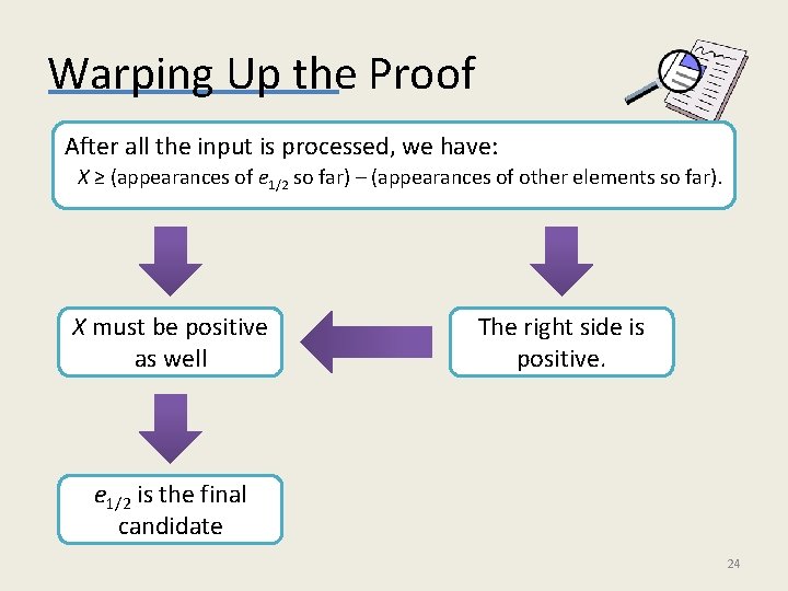
Warping Up the Proof After all the input is processed, we have: X ≥ (appearances of e 1/2 so far) – (appearances of other elements so far). X must be positive as well The right side is positive. e 1/2 is the final candidate 24
Streaming Algorithms for Graph Problems Streaming for Graph Problems • The stream consists of the edges of the graph. • Allows O(n polylog(n)) space. Sublinear in the length of the (Trivial) Algorithm for Counting Connected Components stream which can be ϴ(n 2). 1. Initially each node is an independent connected component. 2. For each edge e that arrives, if the end points of e belong to different connected component, merge these connected components. 25
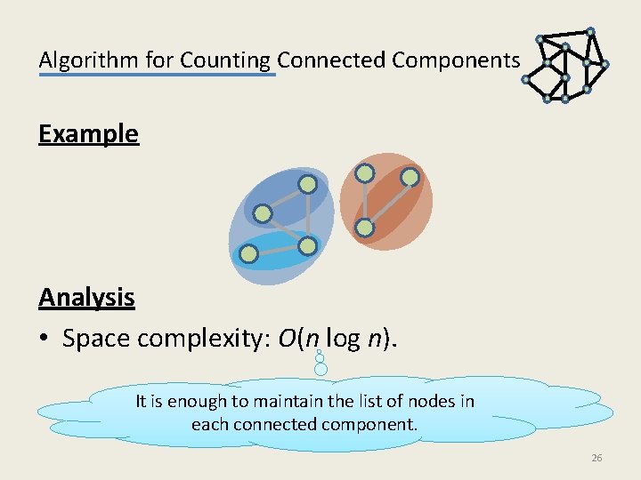
Algorithm for Counting Connected Components Example Analysis • Space complexity: O(n log n). It is enough to maintain the list of nodes in each connected component. 26
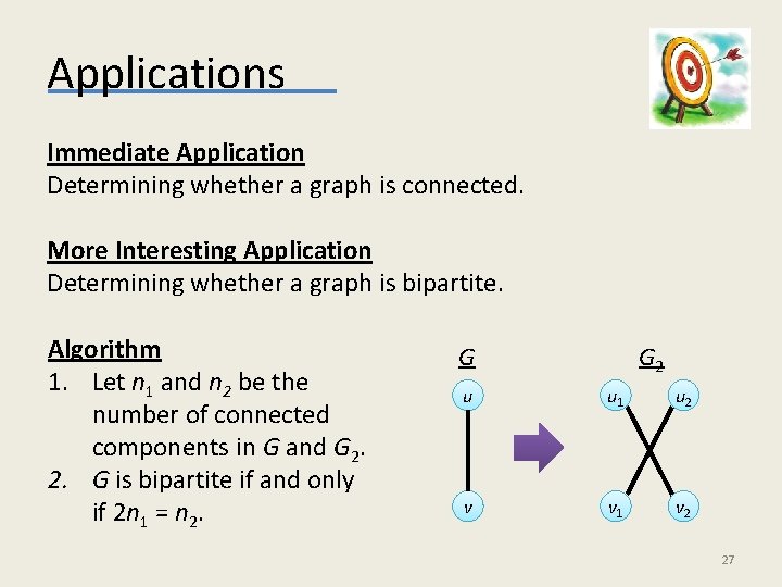
Applications Immediate Application Determining whether a graph is connected. More Interesting Application Determining whether a graph is bipartite. Algorithm 1. Let n 1 and n 2 be the number of connected components in G and G 2. 2. G is bipartite if and only if 2 n 1 = n 2. G G 2 u u 1 u 2 v v 1 v 2 27
Analysis Lemma The copies of the nodes of a connected component C of G form: • Two connected components of G 2 if C is bipartite. • A single connected component of G 2 if C is not bipartite. Proof This alemma that the algorithm is which are not • There is never path inimplies G 2 between copies of nodes correct. connected in G. • If u and v are connected in G, then each copy of u in G 2 is connected to some copy of v. • The copies of the nodes of a connected component C of G form one or two connected components in G 2. Moreover, in the later case each component contains exactly one copy of each node of C. 28
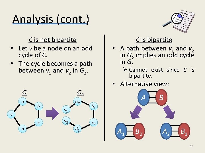
Analysis (cont. ) C is not bipartite • Let v be a node on an odd cycle of C. • The cycle becomes a path between v 1 and v 2 in G 2. C is bipartite • A path between v 1 and v 2 in G 2 implies an odd cycle in G. Ø Cannot exist since C is bipartite. • Alternative view: G a G 2 b v c d a 2 v 1 v 2 d 1 A B b 1 c 2 A 1 B 2 A 2 B 1 29

- Slides: 30