Algorithms for a large sparse nonlinear eigenvalue problem

Algorithms for a large sparse nonlinear eigenvalue problem Yusaku Yamamoto Dept. of Computational Science & Engineering Nagoya University

Outline n n Introduction Algorithms n n n Multivariate Newton’s method Use of the linear eigenvalue of smallest modulus Use of the signed smallest singular value Numerical experiments Conclusion

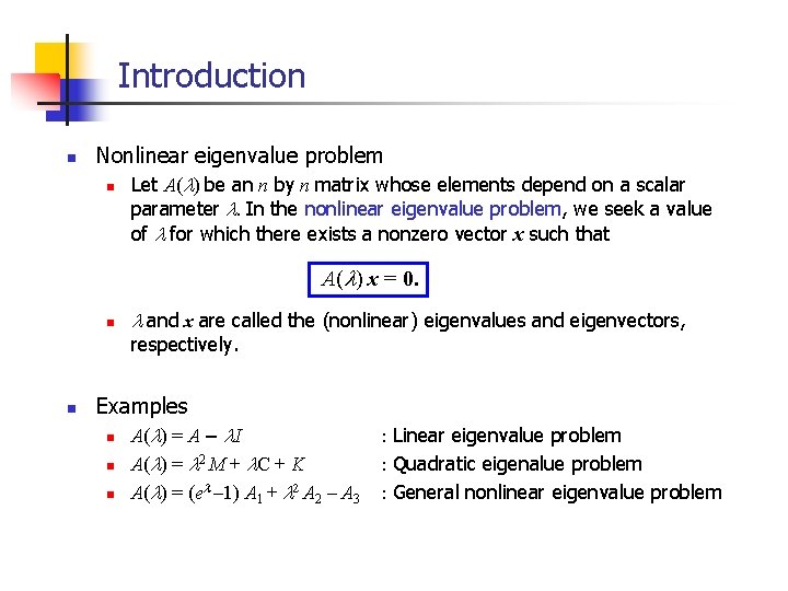
Introduction n Nonlinear eigenvalue problem n Let A(l) be an n by n matrix whose elements depend on a scalar parameter l. In the nonlinear eigenvalue problem, we seek a value of l for which there exists a nonzero vector x such that A(l) x = 0. n l and x are called the (nonlinear) eigenvalues and eigenvectors, respectively. n Examples n A(l) = A – l. I 2 n A(l) = l M + l. C + K l 2 n A(l) = (e – 1) A 1 + l A 2 – A 3 : Linear eigenvalue problem : Quadratic eigenalue problem : General nonlinear eigenvalue problem

Applications of the nonlinear eigenvalue problem n Structural mechanics n Decay system: l 2 Mx + l. Cx + Kx = 0 n n Electronic structure calculation n n M : mass matrix, C : damping matrix, K : stiffness matrix Kohn-Sham equation: H(l)f = lf n H(l): Kohn-Sham Hamiltonian Theoretical fluid dynamics n Computation of the scaling exponent in turbulent flow

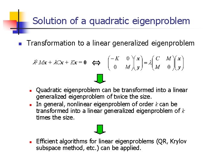
Solution of a quadratic eigenproblem n Transformation to a linear generalized eigenproblem l 2 Mx + l. Cx + Kx = 0 n n n Quadratic eigenproblem can be transformed into a linear generalized eigenproblem of twice the size. In general, nonlinear eigenproblem of order k can be transformed into a linear generalized eigenproblem of k times the size. Efficient algorithms for linear eigenproblems (QR, Krylov subspace method, etc. ) can be applied.

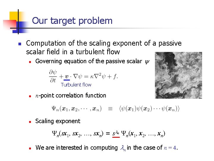
Our target problem n Computation of the scaling exponent of a passive scalar field in a turbulent flow n Governing equation of the passive scalar y Turbulent flow n n-point correlation function n Scaling exponent Yn(sx 1, sx 2, …, sxn) = sln Yn(x 1, x 2, …, xn) n We are interested in computing ln in the case of n = 4.

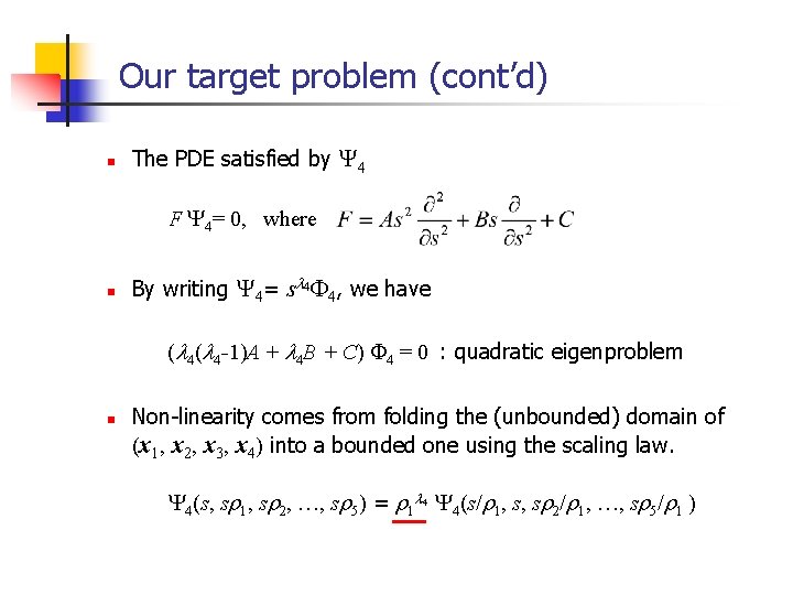
Our target problem (cont’d) n The PDE satisfied by Y 4 F Y 4= 0, where n By writing Y 4= sl 4 F 4, we have (l 4 -1)A + l 4 B + C) F 4 = 0 : quadratic eigenproblem n Non-linearity comes from folding the (unbounded) domain of (x 1, x 2, x 3, x 4) into a bounded one using the scaling law. Y 4(s, sr 1, sr 2, …, sr 5) = r 1 l 4 Y 4(s/r 1, s, sr 2/r 1, …, sr 5/r 1 )

Our target problem (cont’d) n Problem characteristics n n A(l) is large (n ~ 105), sparse and nonsymmetric. Dependence of A(l) on l is fully nonlinear (includes both exponential and polynomial terms in l), but is analytical. Computation of A(l) takes a long time. The smallest positive eigenvalue is sought.

Solution of a general nonlinear eigenproblem n Necessary and sufficient condition for l x 0, A(l) x = 0 n A simple approach (Gat et al. , 1997; the case of n = 3) n Find the solution l of det(A(l)) = 0 by Newton’s method. n n det(A(l)) = 0 Find the eigenvector x as the null space of a constant matrix A(l). Difficulty n n Computation of det(A(l)) requires roughly the same cost as the LU decomposition of A(l). Not efficient when A(l) is large and sparse.

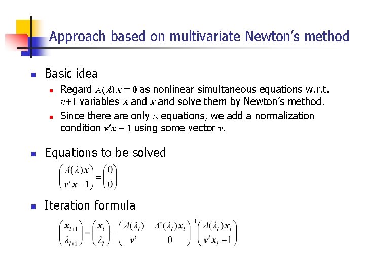
Approach based on multivariate Newton’s method n Basic idea n n Regard A(l) x = 0 as nonlinear simultaneous equations w. r. t. n+1 variables l and x and solve them by Newton’s method. Since there are only n equations, we add a normalization condition vtx = 1 using some vector v. n Equations to be solved n Iteration formula

Multivariate Newton’s method (cont’d) n Advantages n n n Each iteration consists of solving linear simultaneous equations. n Much cheaper than computing det(A(l)). Convergence is quadratic if the initial values l 0 and x 0 are sufficiently close to the solution. Disadvantages n The iterates may converge to unwanted eigenpairs or fail to converge unless both l 0 and x 0 are sufficiently good. n n It is in general difficult to find a good initial value x 0 for the eigenvector. A'(l) is necessary in addition to A(l).

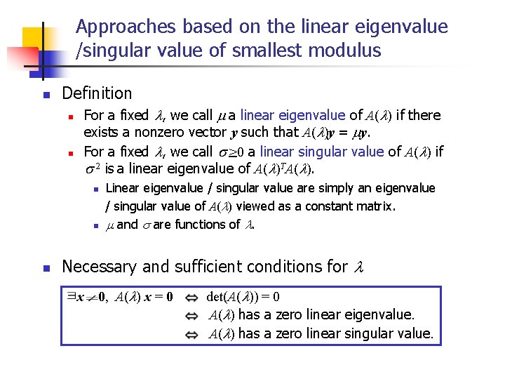
Approaches based on the linear eigenvalue /singular value of smallest modulus n Definition n n For a fixed l, we call m a linear eigenvalue of A(l) if there exists a nonzero vector y such that A(l)y = my. For a fixed l, we call s >0 a linear singular value of A(l) if s 2 is a linear eigenvalue of A(l)TA(l). n n n Linear eigenvalue / singular value are simply an eigenvalue / singular value of A(l) viewed as a constant matrix. m and s are functions of l. Necessary and sufficient conditions for l x 0, A(l) x = 0 det(A(l)) = 0 A(l) has a zero linear eigenvalue. A(l) has a zero linear singular value.

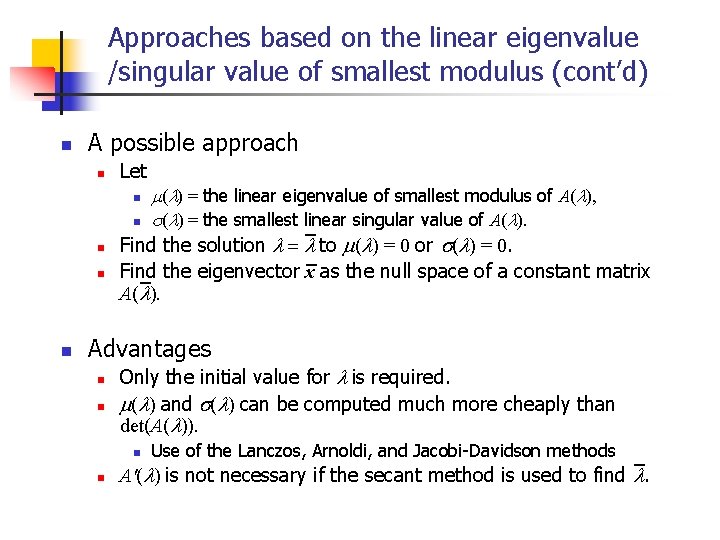
Approaches based on the linear eigenvalue /singular value of smallest modulus (cont’d) n A possible approach n Let n m(l) = the linear eigenvalue of smallest modulus of A(l), n s(l) = the smallest linear singular value of A(l). Find the solution l = l to m(l) = 0 or s(l) = 0. Find the eigenvector x as the null space of a constant matrix A(l). n n n Advantages n n Only the initial value for l is required. m(l) and s(l) can be computed much more cheaply than det(A(l)). n n Use of the Lanczos, Arnoldi, and Jacobi-Davidson methods A'(l) is not necessary if the secant method is used to find l.

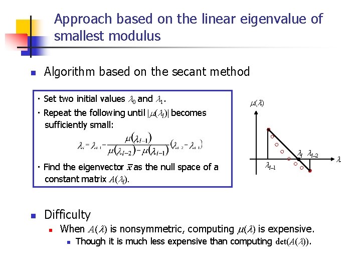
Approach based on the linear eigenvalue of smallest modulus n Algorithm based on the secant method ・ Set two initial values l 0 and l 1. ・ Repeat the following until |m(ll)| becomes sufficiently small: m (l ) ll ll– 2 ・ Find the eigenvector x as the null space of a constant matrix A(ll). n ll– 1 Difficulty n When A(l) is nonsymmetric, computing m(l) is expensive. n Though it is much less expensive than computing det(A(l)). l

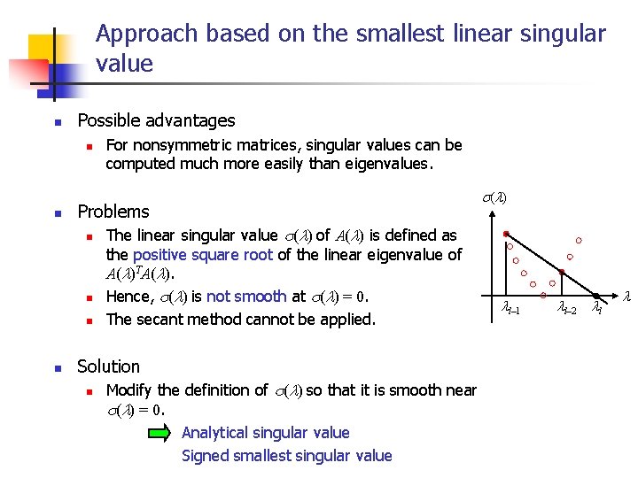
Approach based on the smallest linear singular value n Possible advantages n n Problems n n For nonsymmetric matrices, singular values can be computed much more easily than eigenvalues. The linear singular value s(l) of A(l) is defined as the positive square root of the linear eigenvalue of A(l)TA(l). Hence, s(l) is not smooth at s(l) = 0. The secant method cannot be applied. Solution n Modify the definition of s(l) so that it is smooth near s(l) = 0. Analytical singular value Signed smallest singular value s (l ) ll– 1 ll– 2 ll l

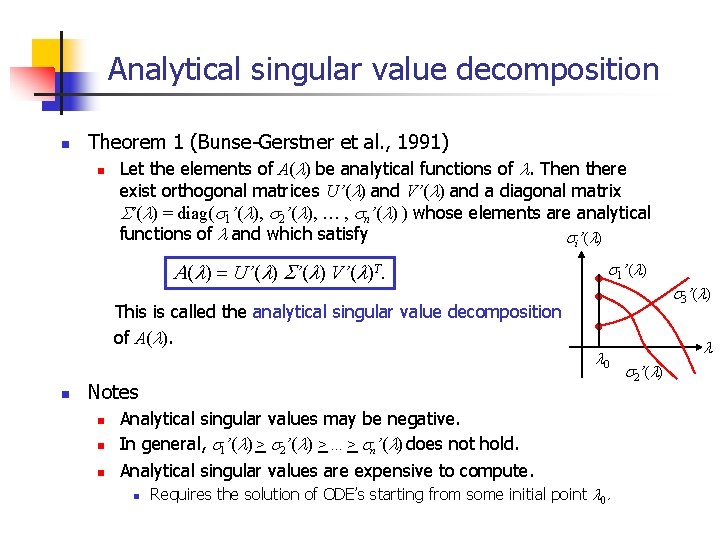
Analytical singular value decomposition n Theorem 1 (Bunse-Gerstner et al. , 1991) n Let the elements of A(l) be analytical functions of l. Then there exist orthogonal matrices U’(l) and V’(l) and a diagonal matrix S’(l) = diag(s 1’(l), s 2’(l), … , sn’(l) ) whose elements are analytical functions of l and which satisfy si’(l) A(l) = U’(l) S’(l) V’(l)T. This is called the analytical singular value decomposition of A(l). n s 1’(l) s 3’(l) l 0 Notes n n n Analytical singular values may be negative. In general, s 1’(l) > s 2’(l) >. . . > sn’(l) does not hold. Analytical singular values are expensive to compute. n Requires the solution of ODE’s starting from some initial point l 0. l s 2’(l)

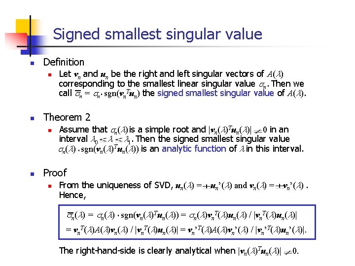
Signed smallest singular value n Definition n n Theorem 2 n n Let vn and un be the right and left singular vectors of A(l) corresponding to the smallest linear singular value sn. Then we call sn = sn. sgn(vn. Tun) the signed smallest singular value of A(l). Assume that sn(l) is a simple root and |vn(l)Tun(l)| 0 in an interval l 0 l l 1. Then the signed smallest singular value sn(l). sgn(vn(l)Tun(l)) is an analytic function of l in this interval. Proof n From the uniqueness of SVD, un(l) = Hence, un’(l) and vn(l) = vn’(l). sn(l) = sn(l). sgn(vn(l)Tun(l)) = sn(l)vn. T(l)un(l) / |vn. T(l)un(l)| = vn. T(l)A(l)vn(l) / |vn. T(l)un(l)| = vn’T(l)A(l)vn’(l) / |vn’T(l)un’(l)|. The right-hand-side is clearly analytical when |vn(l)Tun(l)| 0.

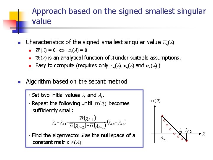
Approach based on the signed smallest singular value n n Characteristics of the signed smallest singular value sn(l) n s n (l ) = 0 n sn(l) is an analytical function of l under suitable assumptions. n Easy to compute (requires only sn(l), vn(l) and un(l) ) Algorithm based on the secant method ・ Set two initial values l 0 and l 1. ・ Repeat the following until |s (ll)| becomes sufficiently small: ・ Find the eigenvector x as the null space of a constant matrix A(ll). s (l ) ll ll– 2 ll– 1 l

Numerical experiments n Test problem n n n Computation of the scaling exponent in turbulent flow Matrix size is 35, 000 and 100, 000. Seek the smallest positive (nonlinear) eigenvalue It is known that the eigenvalue is in [0, 4], but the estimate for the (nonlinear) eigenvector is unknown. Computational environment n Fujitsu Prime. Power HPC 2500 (16 PU)

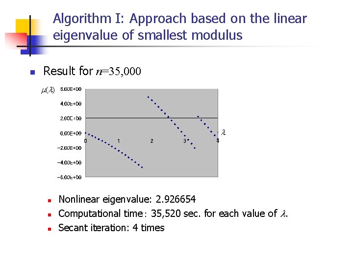
Algorithm I: Approach based on the linear eigenvalue of smallest modulus n Result for n=35, 000 m (l ) l n n n Nonlinear eigenvalue: 2. 926654 Computational time： 35, 520 sec. for each value of l. Secant iteration: 4 times

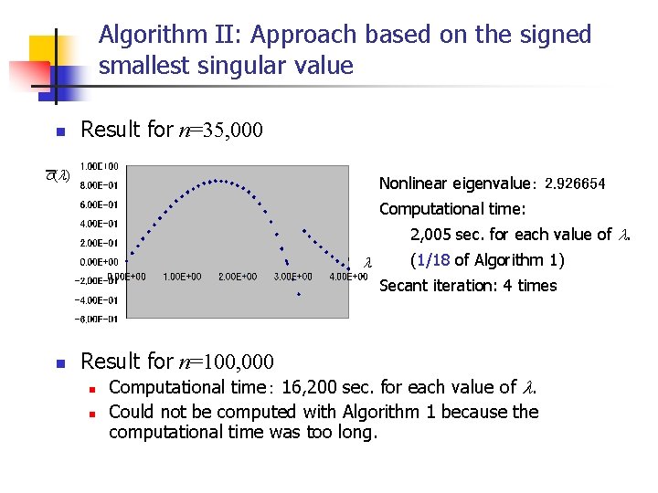
Algorithm II: Approach based on the signed smallest singular value n Result for n=35, 000 s (l ) Nonlinear eigenvalue： 2. 926654 Computational time: 2, 005 sec. for each value of l. l (1/18 of Algorithm 1) Secant iteration: 4 times n Result for n=100, 000 n n Computational time： 16, 200 sec. for each value of l. Could not be computed with Algorithm 1 because the computational time was too long.

Conclusion n Summary of this study n n n We proposed an algorithm for large sparse nonlinear eigenproblem based on the signed smallest positive singular value. The algorithm proved much faster than the method based on the linear eigenvalue of smallest modulus. Future work n Application of the algorithm to various nonlinear eigenproblems