Algorithms Algorithm Techniques Steps in Designing Algorithms1 1

Algorithms Algorithm Techniques

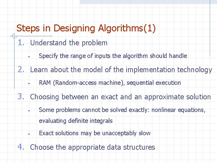
Steps in Designing Algorithms(1) 1. Understand the problem • Specify the range of inputs the algorithm should handle 2. Learn about the model of the implementation technology • RAM (Random-access machine), sequential execution 3. Choosing between an exact and an approximate solution • Some problems cannot be solved exactly: nonlinear equations, evaluating definite integrals • Exact solutions may be unacceptably slow 4. Choose the appropriate data structures

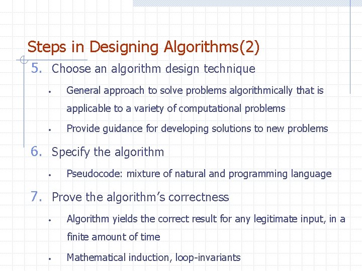
Steps in Designing Algorithms(2) 5. Choose an algorithm design technique • General approach to solve problems algorithmically that is applicable to a variety of computational problems • Provide guidance for developing solutions to new problems 6. Specify the algorithm • Pseudocode: mixture of natural and programming language 7. Prove the algorithm’s correctness • Algorithm yields the correct result for any legitimate input, in a finite amount of time • Mathematical induction, loop-invariants

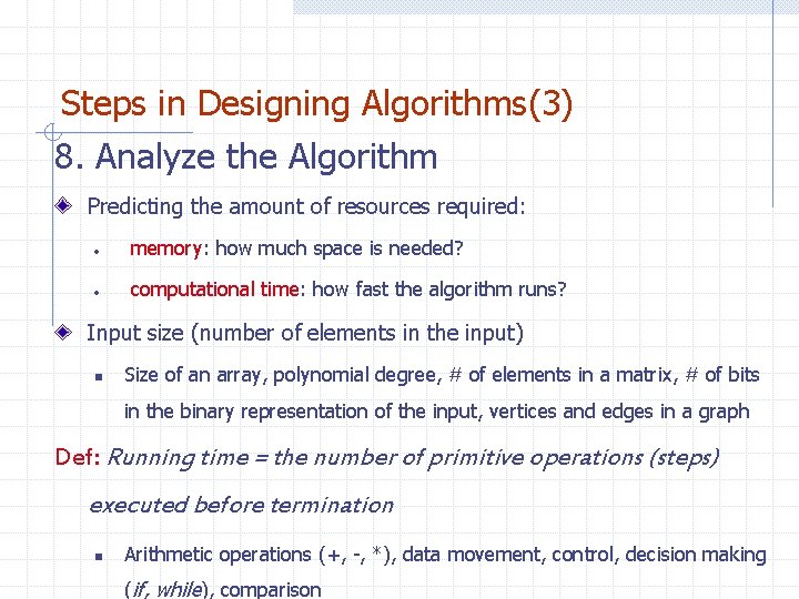
Steps in Designing Algorithms(3) 8. Analyze the Algorithm Predicting the amount of resources required: • memory: how much space is needed? • computational time: how fast the algorithm runs? Input size (number of elements in the input) n Size of an array, polynomial degree, # of elements in a matrix, # of bits in the binary representation of the input, vertices and edges in a graph Def: Running time = the number of primitive operations (steps) executed before termination n Arithmetic operations (+, -, *), data movement, control, decision making (if, while), comparison

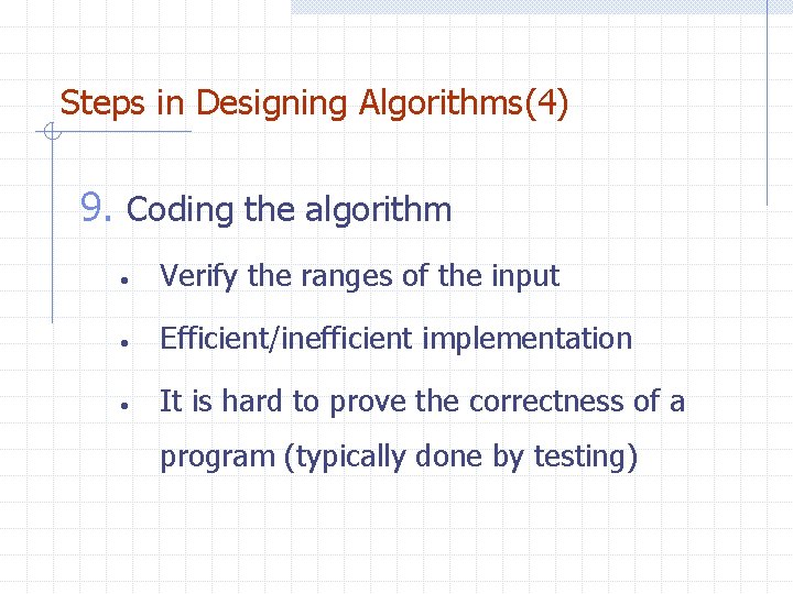
Steps in Designing Algorithms(4) 9. Coding the algorithm • Verify the ranges of the input • Efficient/inefficient implementation • It is hard to prove the correctness of a program (typically done by testing)

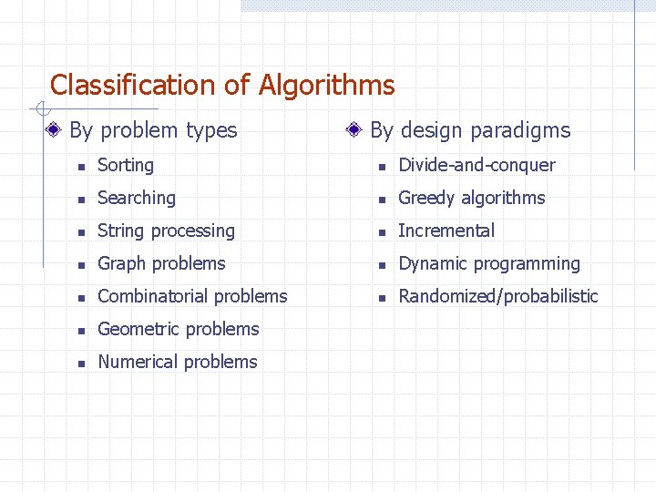
Classification of Algorithms By problem types By design paradigms n Sorting n Divide-and-conquer n Searching n Greedy algorithms n String processing n Incremental n Graph problems n Dynamic programming n Combinatorial problems n Randomized/probabilistic n Geometric problems n Numerical problems

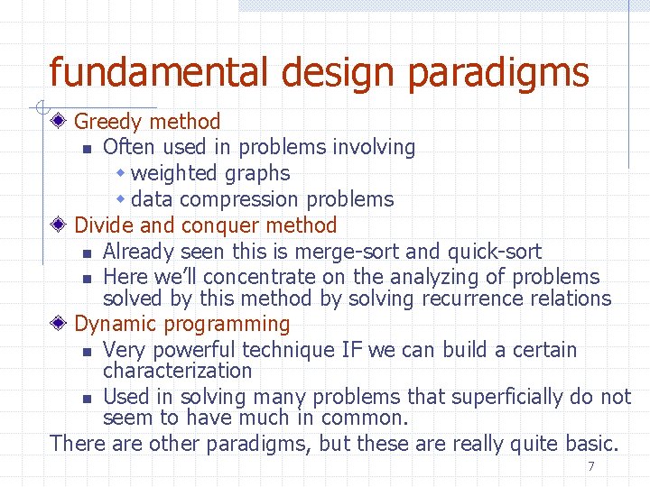
fundamental design paradigms Greedy method n Often used in problems involving w weighted graphs w data compression problems Divide and conquer method n Already seen this is merge-sort and quick-sort n Here we’ll concentrate on the analyzing of problems solved by this method by solving recurrence relations Dynamic programming n Very powerful technique IF we can build a certain characterization n Used in solving many problems that superficially do not seem to have much in common. There are other paradigms, but these are really quite basic. 7

The Greedy Method

Greedy algorithms Suppose it is possible to build a solution through a sequence of partial solutions n At each step, we focus on one particular partial solution and we attempt to extend that solution n Ultimately, the partial solutions should lead to a feasible solution which is also optimal

The Greedy Method Technique The greedy method is a general algorithm design paradigm, built on the following elements: n configurations: different choices, collections, or values to find n an objective function: a score assigned to configurations, which we want to either maximize or minimize n A globally-optimal solution can always be found by a series of local improvements from a starting configuration. 10

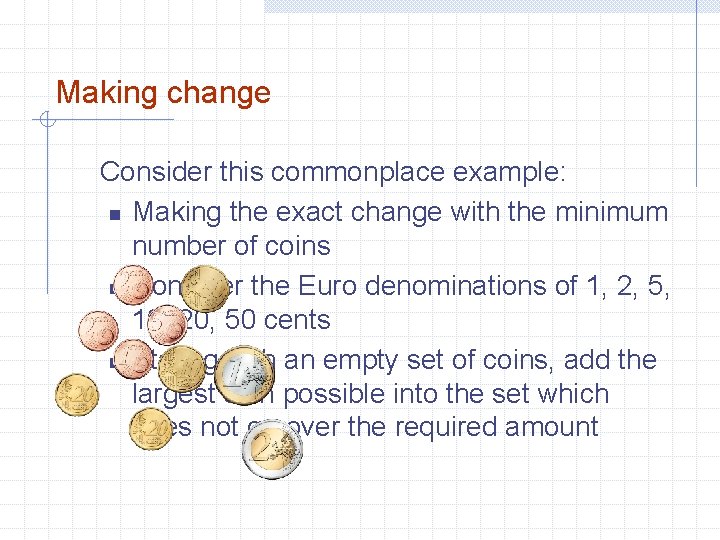
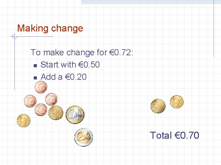
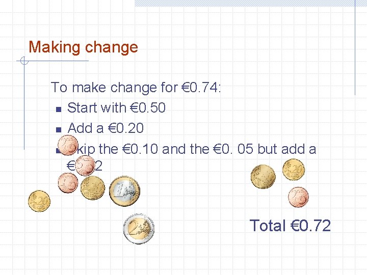
Making change Consider this commonplace example: n Making the exact change with the minimum number of coins n Consider the Euro denominations of 1, 2, 5, 10, 20, 50 cents n Stating with an empty set of coins, add the largest coin possible into the set which does not go over the required amount

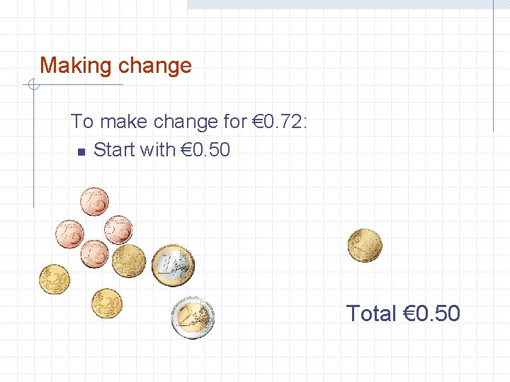
Making change To make change for € 0. 72: n Start with € 0. 50 Total € 0. 50

Making change To make change for € 0. 72: n Start with € 0. 50 n Add a € 0. 20 Total € 0. 70

Making change To make change for € 0. 74: n Start with € 0. 50 n Add a € 0. 20 n Skip the € 0. 10 and the € 0. 05 but add a € 0. 02 Total € 0. 72

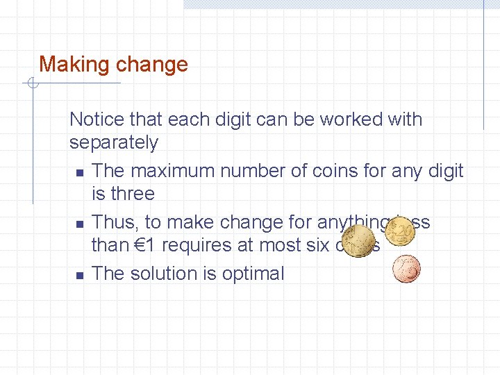
Making change Notice that each digit can be worked with separately n The maximum number of coins for any digit is three n Thus, to make change for anything less than € 1 requires at most six coins n The solution is optimal

Definition A greedy algorithm is an algorithm which has: n A set of partial solutions from which a solution is built n An objective function which assigns a value to any partial solution Then given a partial solution, we n Consider possible extensions of the partial solution n Discard any extensions which are not feasible n Choose that extension which minimizes the object function

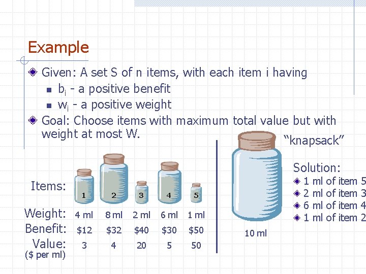
Example Given: A set S of n items, with each item i having n bi - a positive benefit n wi - a positive weight Goal: Choose items with maximum total value but with weight at most W. “knapsack” Solution: Items: Weight: Benefit: Value: ($ per ml) 1 2 3 4 5 4 ml 8 ml 2 ml 6 ml 1 ml $12 $32 $40 $30 $50 3 4 20 5 50 1 2 6 1 10 ml ml ml of of item 5 3 4 2

Problems That Can Be Solved by the Greedy Method A game like chess can be won by thinking ahead. But, a player focusing entirely on their immediate advantage is usually easy to defeat. For example, in Scrabble, the player can do quite well by simply making whatever move seems best at the moment and not worrying about future consequences. 18

On each step in the algorithm, the choice must be: Feasible - i. e. it satisfies the problems constraints Locally optimal – i. e. it has to be the best local choice among all feasible choices available at the step Irrevocable – i. e. once made, it cannot be changed on subsequent steps of the algorithm 19

Example: Making Change Problem: A dollar amount to reach and a collection of coin amounts to use to get there. Configuration: A dollar amount to return to a customer plus the coins already returned Objective function: Minimize number of coins returned. Greedy solution: Always return the largest coin you can 20

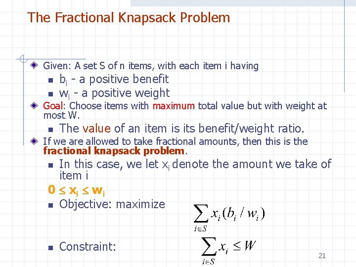
The Fractional Knapsack Problem Given: A set S of n items, with each item i having n n bi - a positive benefit wi - a positive weight Goal: Choose items with maximum total value but with weight at most W. n The value of an item is its benefit/weight ratio. If we are allowed to take fractional amounts, then this is the fractional knapsack problem. In this case, we let xi denote the amount we take of item i 0 xi wi n Objective: maximize n n Constraint: 21

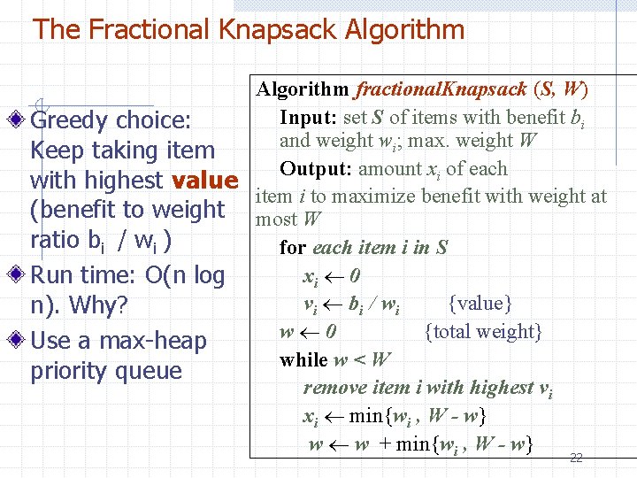
The Fractional Knapsack Algorithm fractional. Knapsack (S, W) Input: set S of items with benefit bi Greedy choice: and weight wi; max. weight W Keep taking item Output: amount xi of each with highest value item i to maximize benefit with weight at (benefit to weight most W ratio bi / wi ) for each item i in S xi 0 Run time: O(n log vi bi / wi {value} n). Why? w 0 {total weight} Use a max-heap while w < W priority queue remove item i with highest vi xi min{wi , W - w} w w + min{wi , W - w} 22

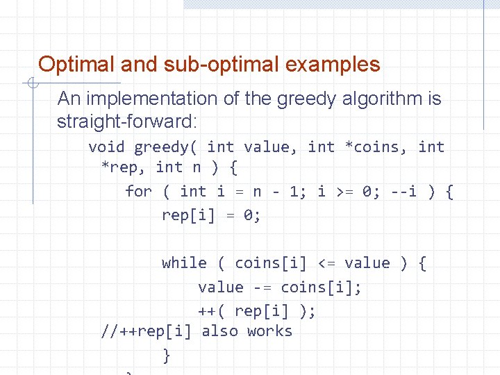
Optimal and sub-optimal examples An implementation of the greedy algorithm is straight-forward: void greedy( int value, int *coins, int *rep, int n ) { for ( int i = n - 1; i >= 0; --i ) { rep[i] = 0; while ( coins[i] <= value ) { value -= coins[i]; ++( rep[i] ); //++rep[i] also works }

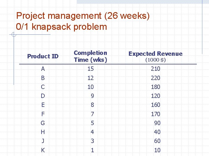
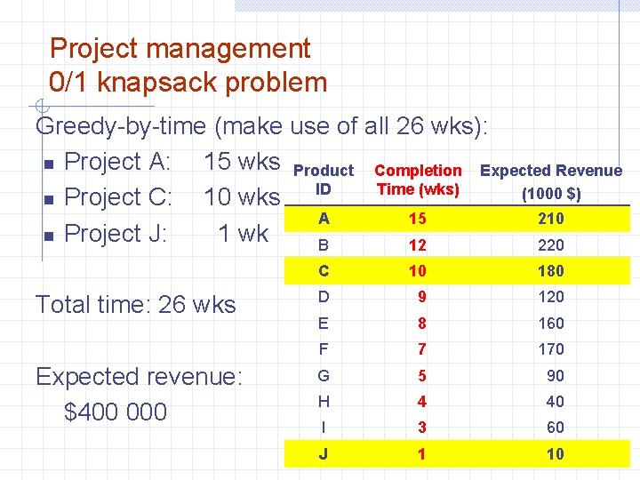
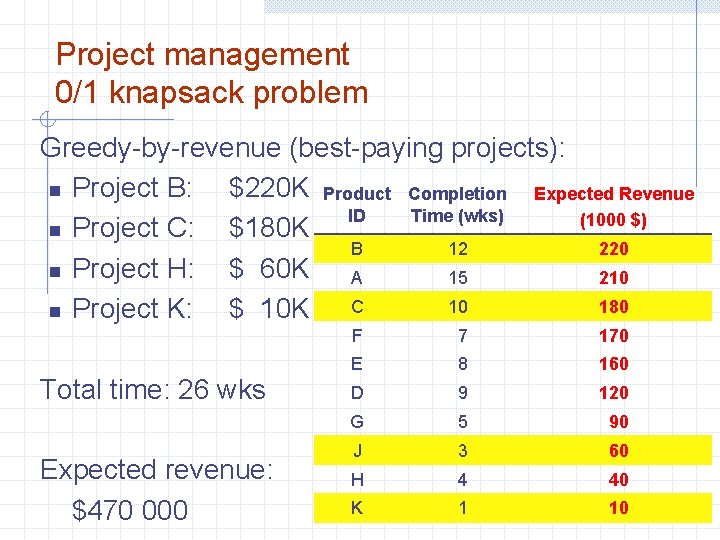
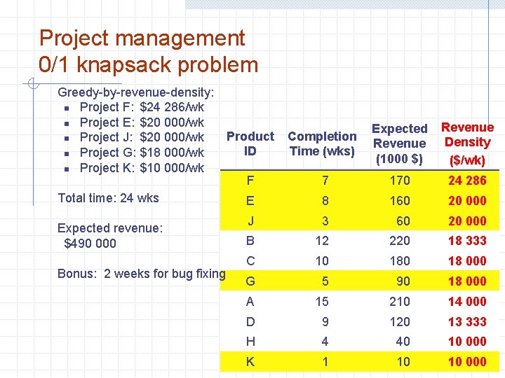
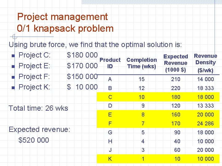
Project management (26 weeks) 0/1 knapsack problem Product ID Completion Time (wks) Expected Revenue A 15 210 B 12 220 C 10 180 D 9 120 E 8 160 F 7 170 G 5 90 H 4 40 J 3 60 K 1 10 (1000 $)

Project management 0/1 knapsack problem Greedy-by-time (make use of all 26 wks): n Project A: 15 wks Product Completion Expected Revenue Time (wks) (1000 $) n Project C: 10 wks ID A 15 210 n Project J: 1 wk B 12 220 Total time: 26 wks Expected revenue: $400 000 C 10 180 D 9 120 E 8 160 F 7 170 G 5 90 H 4 40 I 3 60 J 1 10

Project management 0/1 knapsack problem Greedy-by-revenue (best-paying projects): n Project B: $220 K Product Completion Expected Revenue ID Time (wks) (1000 $) n Project C: $180 K B 12 220 n Project H: $ 60 K A 15 210 10 180 n Project K: $ 10 K C Total time: 26 wks Expected revenue: $470 000 F 7 170 E 8 160 D 9 120 G 5 90 J 3 60 H 4 40 K 1 10

Project management 0/1 knapsack problem Greedy-by-revenue-density: n Project F: $24 286/wk n Project E: $20 000/wk Product n Project J: $20 000/wk ID n Project G: $18 000/wk n Project K: $10 000/wk F Total time: 24 wks E Expected revenue: $490 000 Bonus: 2 weeks for bug fixing Completion Time (wks) Expected Revenue (1000 $) Revenue Density ($/wk) 7 170 24 286 8 160 20 000 J 3 60 20 000 B 12 220 18 333 C 10 18 000 G 5 90 18 000 A 15 210 14 000 D 9 120 13 333 H 4 40 10 000 K 1 10 10 000

Project management 0/1 knapsack problem Using brute force, we find that the optimal solution is: n Project C: $180 000 Expected Product Completion Revenue n Project E: $170 000 ID Time (wks) (1000 $) n Project F: $150 000 A 15 210 n Project K: $ 10 000 B 12 220 Total time: 26 wks Expected revenue: $520 000 Revenue Density ($/wk) 14 000 18 333 C 10 18 000 D 9 120 13 333 E 8 160 20 000 F 7 170 24 286 G 5 90 18 000 H 4 40 10 000 J 3 60 20 000 K 1 10 10 000

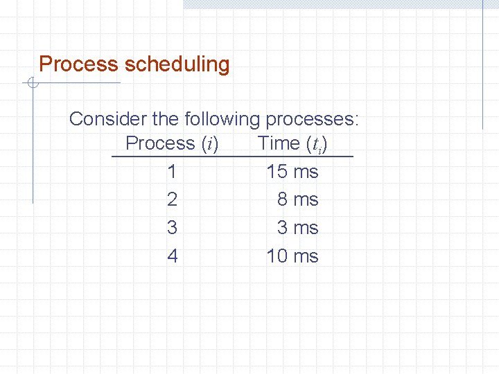
Process scheduling Consider the following processes: Process (i) Time (ti) 1 15 ms 2 8 ms 3 3 ms 4 10 ms

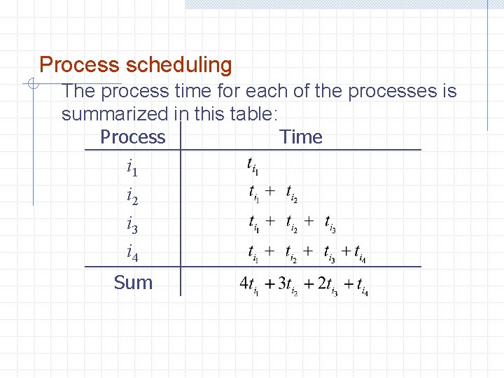
Process scheduling The process time for each of the processes is summarized in this table: Process Time i 1 i 2 i 3 i 4 Sum

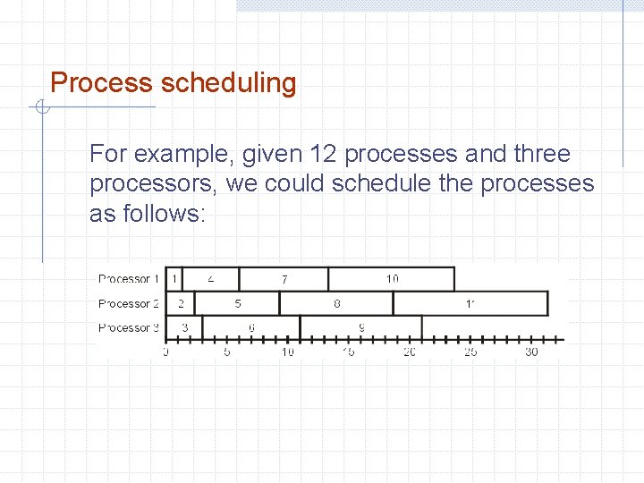
Process scheduling For example, given 12 processes and three processors, we could schedule the processes as follows:

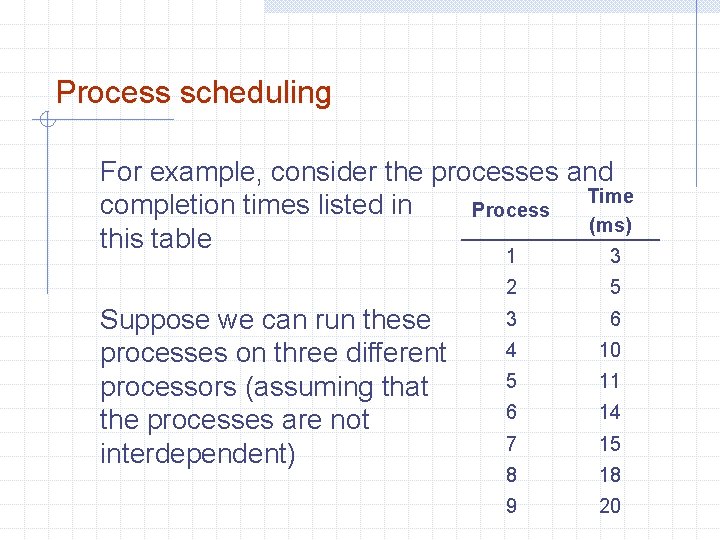
Process scheduling For example, consider the processes and Time completion times listed in Process (ms) this table Suppose we can run these processes on three different processors (assuming that the processes are not interdependent) 1 3 2 5 3 6 4 10 5 11 6 14 7 15 8 18 9 20

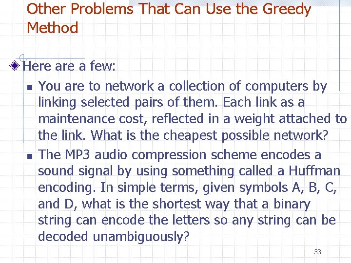
Other Problems That Can Use the Greedy Method Here a few: n You are to network a collection of computers by linking selected pairs of them. Each link as a maintenance cost, reflected in a weight attached to the link. What is the cheapest possible network? n The MP 3 audio compression scheme encodes a sound signal by using something called a Huffman encoding. In simple terms, given symbols A, B, C, and D, what is the shortest way that a binary string can encode the letters so any string can be decoded unambiguously? 33

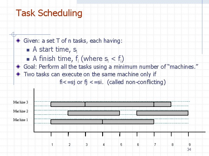
Task Scheduling Given: a set T of n tasks, each having: n n A start time, si A finish time, fi (where si < fi) Goal: Perform all the tasks using a minimum number of “machines. ” Two tasks can execute on the same machine only if fi<=sj or fj <=si. (called non-conflicting) Machine 3 Machine 2 Machine 1 1 2 3 4 5 6 7 8 9 34

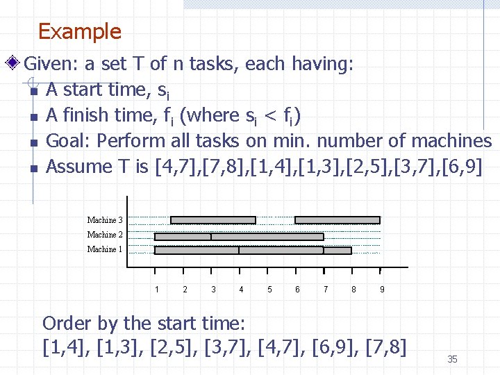
Example Given: a set T of n tasks, each having: n A start time, si n A finish time, fi (where si < fi) n Goal: Perform all tasks on min. number of machines n Assume T is [4, 7], [7, 8], [1, 4], [1, 3], [2, 5], [3, 7], [6, 9] Machine 3 Machine 2 Machine 1 1 2 3 4 5 6 7 8 9 Order by the start time: [1, 4], [1, 3], [2, 5], [3, 7], [4, 7], [6, 9], [7, 8] 35

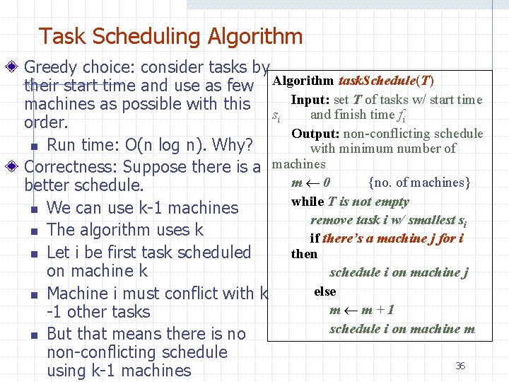
Task Scheduling Algorithm Greedy choice: consider tasks by their start time and use as few Algorithm task. Schedule(T) Input: set T of tasks w/ start time machines as possible with this si and finish time fi order. Output: non-conflicting schedule n Run time: O(n log n). Why? with minimum number of Correctness: Suppose there is a machines m 0 {no. of machines} better schedule. while T is not empty n We can use k-1 machines remove task i w/ smallest si n The algorithm uses k if there’s a machine j for i then n Let i be first task scheduled on machine k schedule i on machine j else n Machine i must conflict with k m m+1 -1 other tasks schedule i on machine m n But that means there is no non-conflicting schedule 36 using k-1 machines

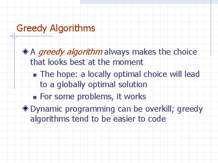
Greedy Algorithms A greedy algorithm always makes the choice that looks best at the moment n The hope: a locally optimal choice will lead to a globally optimal solution n For some problems, it works Dynamic programming can be overkill; greedy algorithms tend to be easier to code

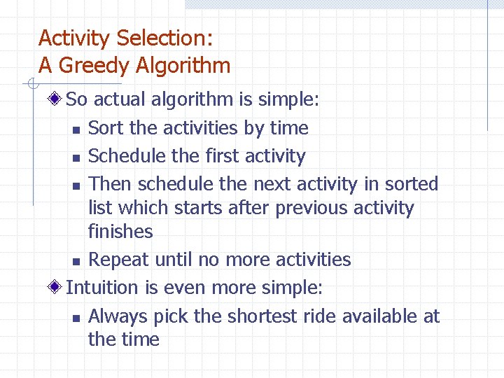
Activity Selection: A Greedy Algorithm So actual algorithm is simple: n Sort the activities by time n Schedule the first activity n Then schedule the next activity in sorted list which starts after previous activity finishes n Repeat until no more activities Intuition is even more simple: n Always pick the shortest ride available at the time

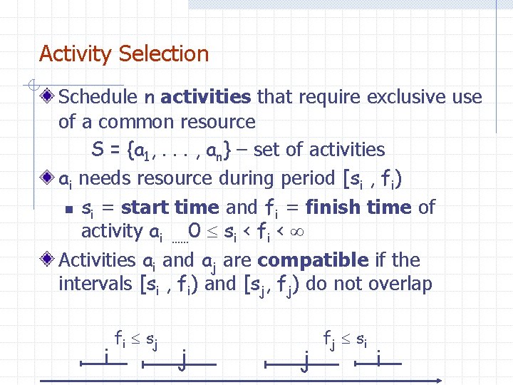
Activity Selection Schedule n activities that require exclusive use of a common resource S = {a 1, . . . , an} – set of activities ai needs resource during period [si , fi) n si = start time and fi = finish time of activity ai …… 0 si < fi < Activities ai and aj are compatible if the intervals [si , fi) and [sj, fj) do not overlap i fi s j j j fj s i i

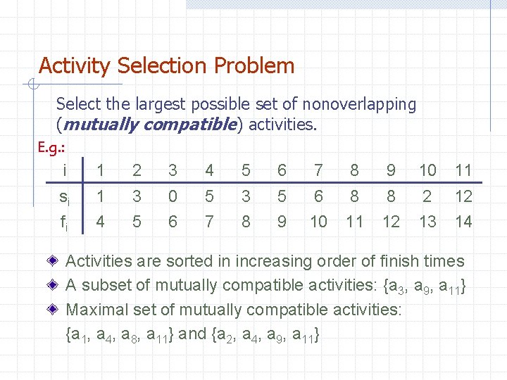
Activity Selection Problem Select the largest possible set of nonoverlapping (mutually compatible) activities. E. g. : i 1 2 3 4 5 6 7 8 9 10 11 si 1 3 0 5 3 5 6 8 8 2 12 fi 4 5 6 7 8 9 10 11 12 13 14 Activities are sorted in increasing order of finish times A subset of mutually compatible activities: {a 3, a 9, a 11} Maximal set of mutually compatible activities: {a 1, a 4, a 8, a 11} and {a 2, a 4, a 9, a 11}

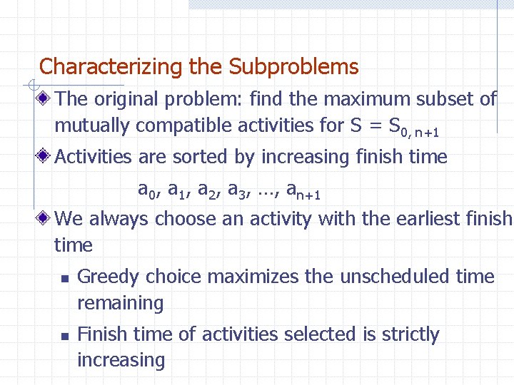
Characterizing the Subproblems The original problem: find the maximum subset of mutually compatible activities for S = S 0, n+1 Activities are sorted by increasing finish time a 0, a 1, a 2, a 3, …, an+1 We always choose an activity with the earliest finish time n n Greedy choice maximizes the unscheduled time remaining Finish time of activities selected is strictly increasing

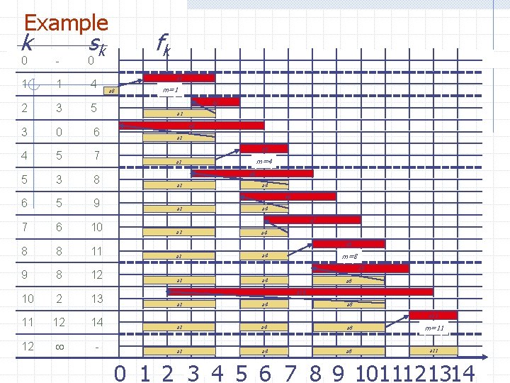
Example k sk 0 - 0 1 1 4 2 3 5 3 0 6 4 5 7 5 3 8 6 5 9 7 6 10 8 8 11 9 8 12 10 2 13 fk a 1 a 0 m=1 a 2 a 1 a 3 a 1 a 4 m=4 a 1 a 5 a 1 a 4 a 6 a 1 a 4 a 7 a 1 a 4 a 8 a 1 m=8 a 4 a 9 a 1 a 4 a 8 a 10 a 1 a 4 a 8 a 11 11 12 14 a 1 a 4 a 8 m=11 12 - a 1 a 4 a 8 a 11 0 1 2 3 4 5 6 7 8 9 1011121314 COSC 3101 A 42

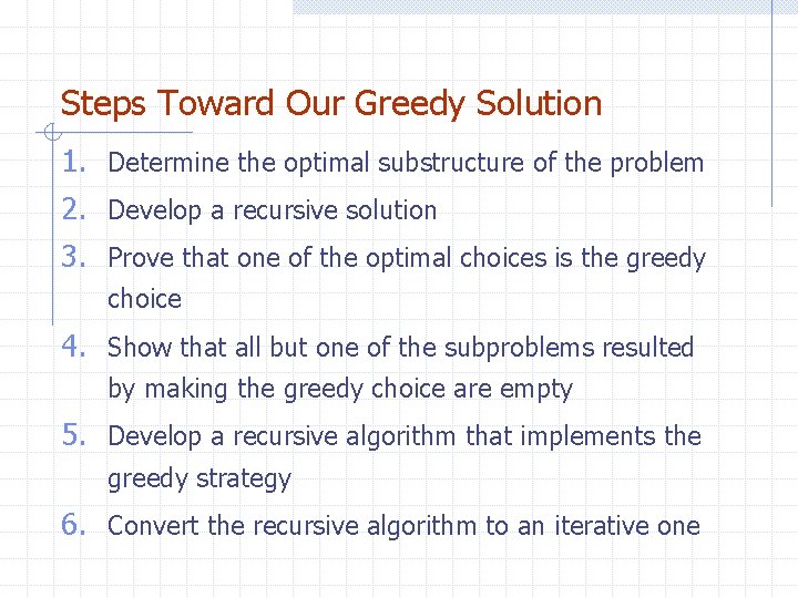
Steps Toward Our Greedy Solution 1. Determine the optimal substructure of the problem 2. Develop a recursive solution 3. Prove that one of the optimal choices is the greedy choice 4. Show that all but one of the subproblems resulted by making the greedy choice are empty 5. Develop a recursive algorithm that implements the greedy strategy 6. Convert the recursive algorithm to an iterative one

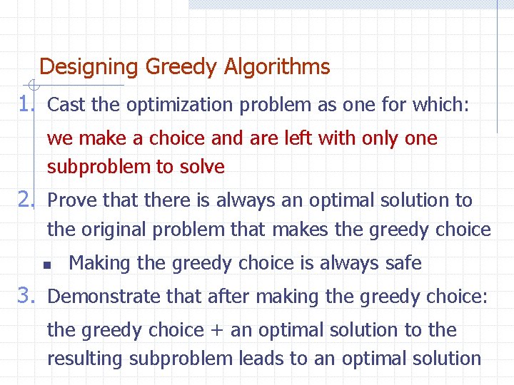
Designing Greedy Algorithms 1. Cast the optimization problem as one for which: we make a choice and are left with only one subproblem to solve 2. Prove that there is always an optimal solution to the original problem that makes the greedy choice n Making the greedy choice is always safe 3. Demonstrate that after making the greedy choice: the greedy choice + an optimal solution to the resulting subproblem leads to an optimal solution

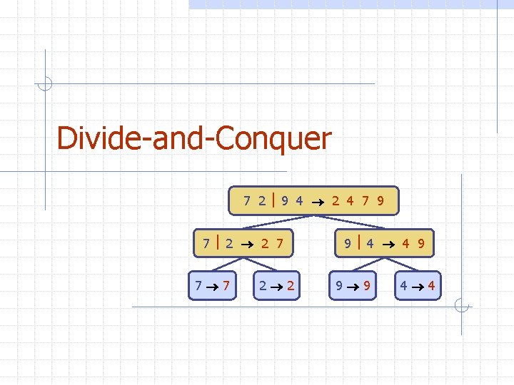
Divide-and-Conquer 7 2 9 4 2 4 7 9 7 2 2 7 7 7 2 2 9 4 4 9 9 9 4 4

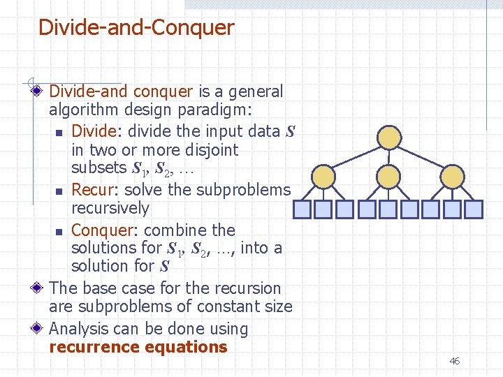
Divide-and-Conquer Divide-and conquer is a general algorithm design paradigm: n Divide: divide the input data S in two or more disjoint subsets S 1, S 2, … n Recur: solve the subproblems recursively n Conquer: combine the solutions for S 1, S 2, …, into a solution for S The base case for the recursion are subproblems of constant size Analysis can be done using recurrence equations 46

Many Problems Fall to Divide and Conquer Mergesort and quicksort were mentioned earlier. Compute gcd (greatest common divisor) of two positive integers. Compute the median of a list of numbers. Multiplying two polynomials of degree 2 d i. e. (1 + 2 x + 3 x^2) * (5 -4 x + 8 x^2) FFT - Fast Fourier Transform used in signal processing. (Closest Pair) Given points in the plane, find two that have the minimum distance between them.

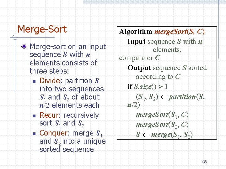
Merge-Sort Merge-sort on an input sequence S with n elements consists of three steps: n Divide: partition S into two sequences S 1 and S 2 of about n/2 elements each n Recur: recursively sort S 1 and S 2 n Conquer: merge S 1 and S 2 into a unique sorted sequence Algorithm merge. Sort(S, C) Input sequence S with n elements, comparator C Output sequence S sorted according to C if S. size() > 1 (S 1, S 2) partition(S, n/2) merge. Sort(S 1, C) merge. Sort(S 2, C) S merge(S 1, S 2) 48

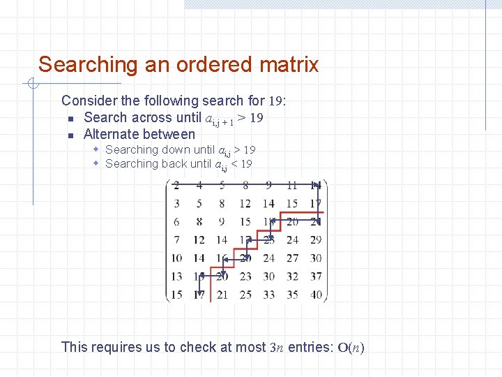
Searching an ordered matrix Consider the following search for 19: n Search across until ai, j + 1 > 19 n Alternate between w Searching down until ai, j > 19 w Searching back until ai, j < 19 This requires us to check at most 3 n entries: O(n)

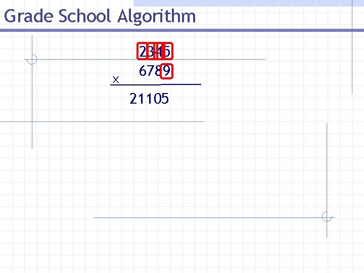
Grade School Algorithm x 2345 6789 21105

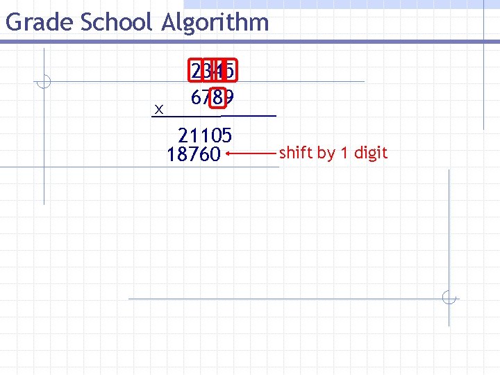
Grade School Algorithm x 2345 6789 21105 18760 shift by 1 digit

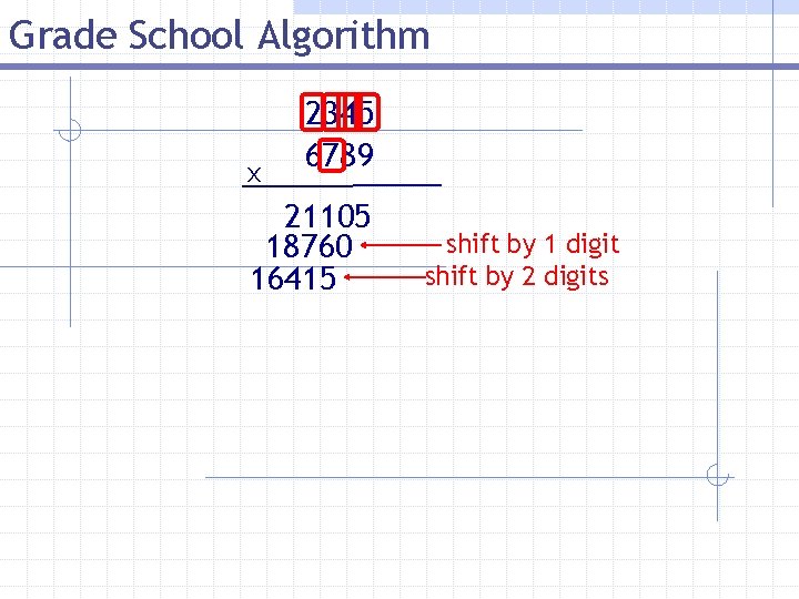
Grade School Algorithm x 2345 6789 21105 18760 16415 shift by 1 digit shift by 2 digits

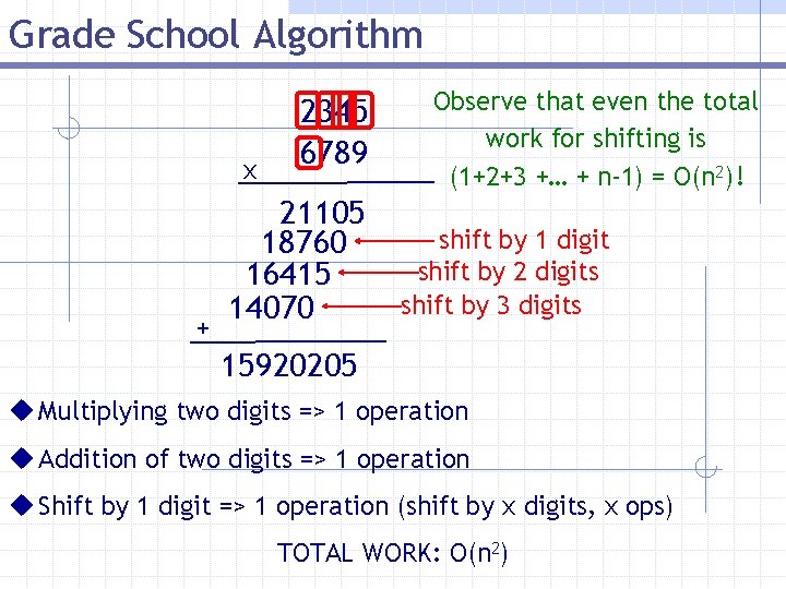
Grade School Algorithm x + 2345 6789 21105 18760 16415 14070 Observe that even the total work for shifting is (1+2+3 +… + n-1) = O(n 2)! shift by 1 digit shift by 2 digits shift by 3 digits 15920205 u Multiplying two digits => 1 operation u Addition of two digits => 1 operation u Shift by 1 digit => 1 operation (shift by x digits, x ops) TOTAL WORK: O(n 2)

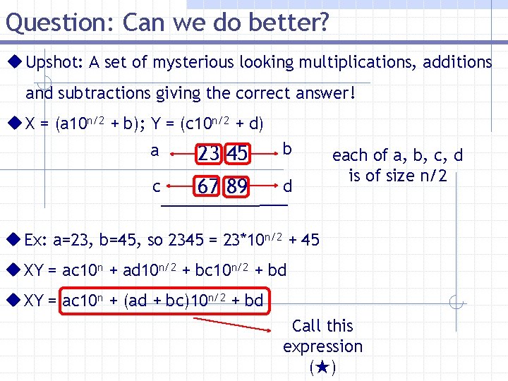
Question: Can we do better? u Upshot: A set of mysterious looking multiplications, additions and subtractions giving the correct answer! u X = (a 10 n/2 + b); Y = (c 10 n/2 + d) a 23 45 b c 67 89 d each of a, b, c, d is of size n/2 u Ex: a=23, b=45, so 2345 = 23*10 n/2 + 45 u XY = ac 10 n + ad 10 n/2 + bc 10 n/2 + bd u XY = ac 10 n + (ad + bc)10 n/2 + bd Call this expression (★)

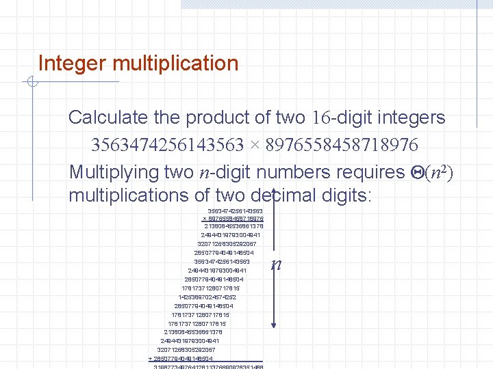
Integer multiplication Calculate the product of two 16 -digit integers 3563474256143563 × 8976558458718976 Multiplying two n-digit numbers requires Q(n 2) multiplications of two decimal digits: 3563474256143563 × 8976558458718976 21380845536861378 24944319793004941 32071268305292067 28507794049148504 3563474256143563 24944319793004941 28507794049148504 17817371280717815 14253897024574252 28507794049148504 17817371280717815 21380845536861378 24944319793004941 32071268305292067 + 28507794049148504. n

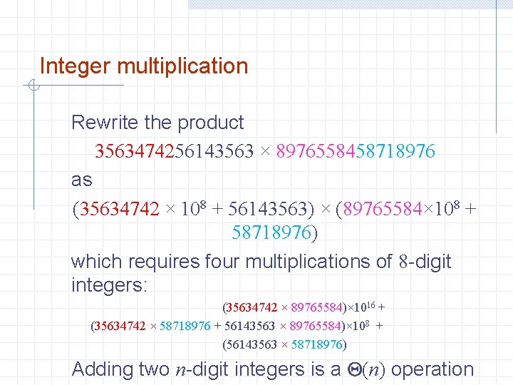
Integer multiplication Rewrite the product 3563474256143563 × 8976558458718976 as (35634742 × 108 + 56143563) × (89765584× 108 + 58718976) which requires four multiplications of 8 -digit integers: (35634742 × 89765584)× 1016 + (35634742 × 58718976 + 56143563 × 89765584)× 108 + (56143563 × 58718976) Adding two n-digit integers is a Q(n) operation

Problem: Big Integer Multiplication Problem: Given two n-bit integers, I and J, that can’t be handled by the hardware of a machine, devise an algorithm with good complexity that multiplies these two numbers. Applications: Encryption schemes used in security work. Can we do better? We will assume n is a power of 2; otherwise, pad with zeroes. Note: This provides an alternate way of doing what we did in the first homework assignment which tacitly assumed the hardware could handle 57 the products.

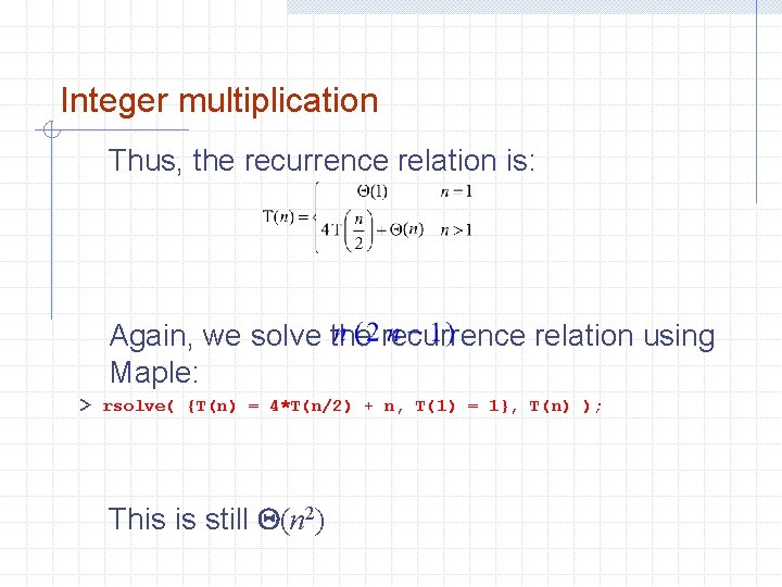
Integer multiplication Thus, the recurrence relation is: Again, we solve the recurrence relation using Maple: > rsolve( {T(n) = 4*T(n/2) + n, T(1) = 1}, T(n) ); This is still Q(n 2)

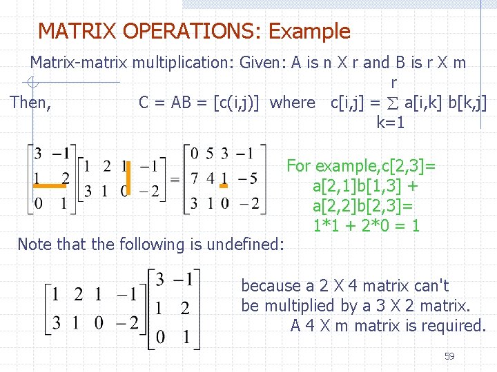
MATRIX OPERATIONS: Example Matrix-matrix multiplication: Given: A is n X r and B is r X m r Then, C = AB = [c(i, j)] where c[i, j] = a[i, k] b[k, j] k=1 Note that the following is undefined: For example, c[2, 3]= a[2, 1]b[1, 3] + a[2, 2]b[2, 3]= 1*1 + 2*0 = 1 because a 2 X 4 matrix can't be multiplied by a 3 X 2 matrix. A 4 X m matrix is required. 59

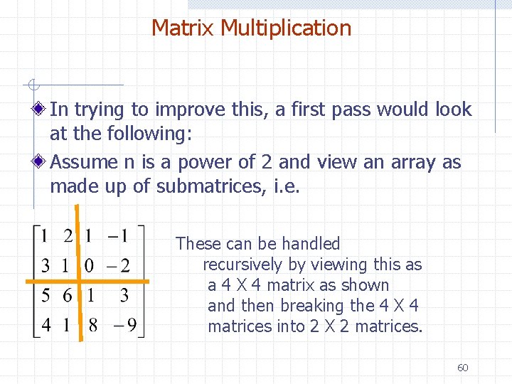
Matrix Multiplication In trying to improve this, a first pass would look at the following: Assume n is a power of 2 and view an array as made up of submatrices, i. e. These can be handled recursively by viewing this as a 4 X 4 matrix as shown and then breaking the 4 X 4 matrices into 2 X 2 matrices. 60

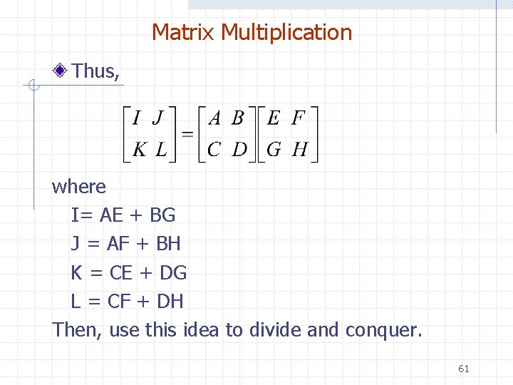
Matrix Multiplication Thus, where I= AE + BG J = AF + BH K = CE + DG L = CF + DH Then, use this idea to divide and conquer. 61

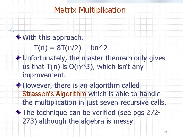
Matrix Multiplication With this approach, T(n) = 8 T(n/2) + bn^2 Unfortunately, the master theorem only gives us that T(n) is O(n^3), which isn't any improvement. However, there is an algorithm called Strassen's Algorithm which is able to handle the multiplication in just seven recursive calls. The technique can be verified (see pgs 272273) although the algebra is messy. 62

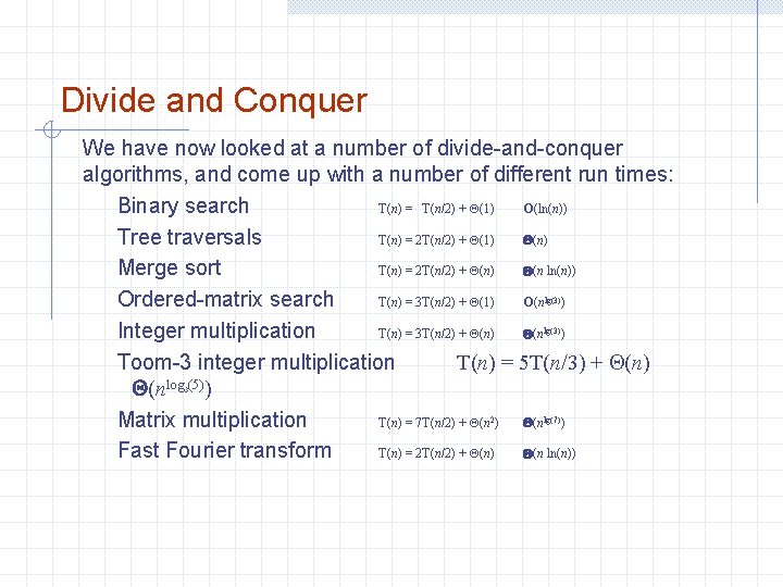
Divide and Conquer We have now looked at a number of divide-and-conquer algorithms, and come up with a number of different run times: Binary search T(n) = T(n/2) + Q(1) O(ln(n)) Tree traversals T(n) = 2 T(n/2) + Q(1) Q(n) Merge sort T(n) = 2 T(n/2) + Q(n) Q(n ln(n)) Ordered-matrix search T(n) = 3 T(n/2) + Q(1) O(n ) Integer multiplication T(n) = 3 T(n/2) + Q(n) Q(n ) Toom-3 integer multiplication T(n) = 5 T(n/3) + Q(n) Q(nlog (5)) Matrix multiplication T(n) = 7 T(n/2) + Q(n ) Fast Fourier transform T(n) = 2 T(n/2) + Q(n) Q(n ln(n)) lg(3) 3 2 lg(7)