Algorithmic patterns Data structures and algorithms in Java

Algorithmic patterns Data structures and algorithms in Java Anastas Misev Parts used by kind permission: • Bruno Preiss, Data Structures and Algorithms with Object-Oriented Design Patterns in Java • David Watt and Deryck F. Brown, Java Collections, An Introduction to Abstract Data Types, Data Structures and Algorithms • Klaus Bothe, Humboldt University Berlin, course Praktische Informatik 1

Algorithmic patterns l l l The notion of algorithmic patterns Algorithmic patterns Problem analyzing Choosing the appropriate pattern Examples Reference: Preiss, ch. 14

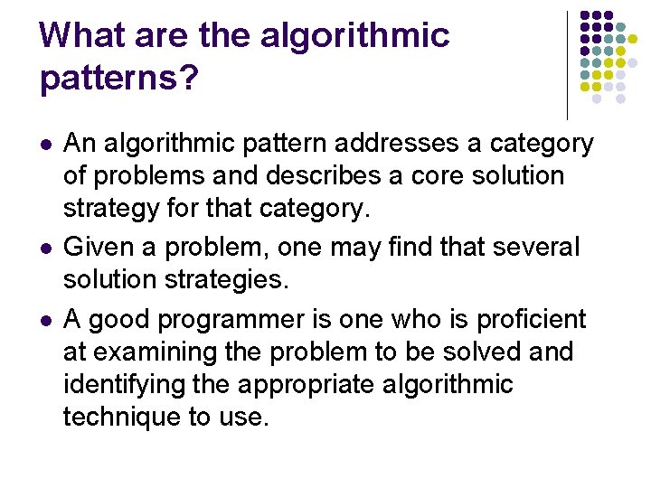
What are the algorithmic patterns? l l l An algorithmic pattern addresses a category of problems and describes a core solution strategy for that category. Given a problem, one may find that several solution strategies. A good programmer is one who is proficient at examining the problem to be solved and identifying the appropriate algorithmic technique to use.

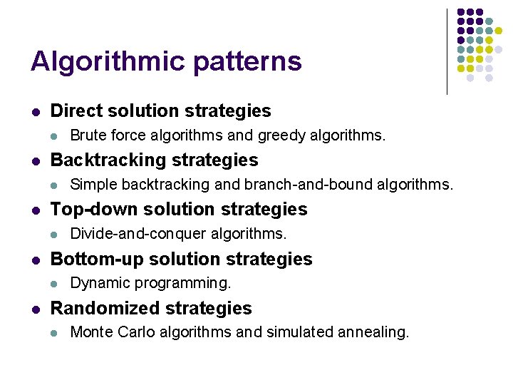
Algorithmic patterns l Direct solution strategies l l Backtracking strategies l l Divide-and-conquer algorithms. Bottom-up solution strategies l l Simple backtracking and branch-and-bound algorithms. Top-down solution strategies l l Brute force algorithms and greedy algorithms. Dynamic programming. Randomized strategies l Monte Carlo algorithms and simulated annealing.

Direct solution strategies l l Brute force Greedy algorithms

Brute force l l l Distinguished not by their structure or form, but by the way in which the problem to be solved is approached. A brute-force algorithm solves a problem in the most simple, direct or obvious way. As a result, such an algorithm can end up doing far more work to solve a given problem than a more clever or sophisticated algorithm might do. On the other hand, a brute-force algorithm is often easier to implement than a more sophisticated one. Exploring all the possible possibilities.

Greedy algorithms l l l Similar to brut force The solution is a sequence of decisions. Once a given decision has been made, that decision is never reconsidered. Greedy algorithms can run significantly faster than brute force ones. Unfortunately, it is not always the case that a greedy strategy leads to the correct solution. l l l Not the right solution Not the best solution Problems – local extremes

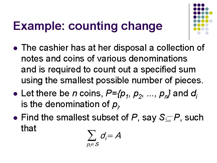
Example: counting change l l l The cashier has at her disposal a collection of notes and coins of various denominations and is required to count out a specified sum using the smallest possible number of pieces. Let there be n coins, P={p 1, p 2, . . . , pn} and di is the denomination of pi. Find the smallest subset of P, say S P, such that

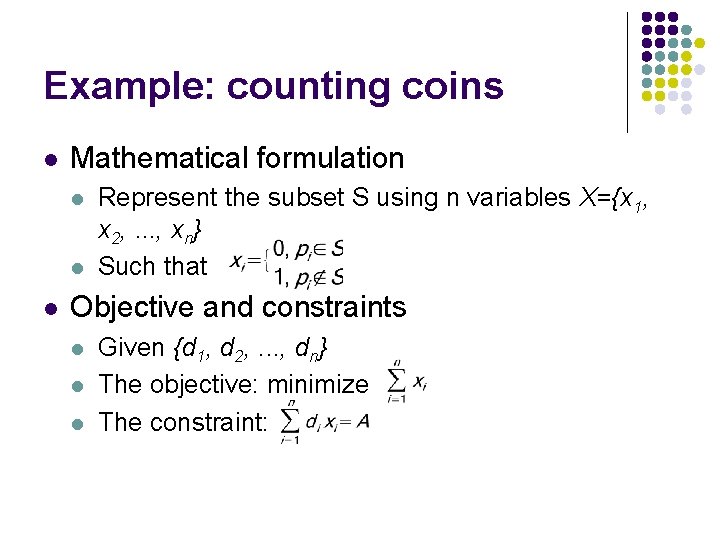
Example: counting coins l Mathematical formulation l l l Represent the subset S using n variables X={x 1, x 2, . . . , xn} Such that Objective and constraints l l l Given {d 1, d 2, . . . , dn} The objective: minimize The constraint:

Brute force solution l l Enumeration all 2 n possible values for X For each value of X check if the constraint is satisfied. A value which satisfies the constraint is called a feasible solution. The solution to the problem is the feasible solution which minimizes the objective function.

Running time l l l There are 2 n possible values of X Therefore running time is (2 n) Running time to determine whether a solution is feasible is O(n) Time to evaluate the objective function is also O(n) Therefore running time O(n 2 n)

Greedy algorithm solution l l l Assume that the pieces of money are sorted by their denomination Count out the amount starting with the largest denomination and proceeding to the smallest denomination. This is greedy because once a coin has been counted out, it is never taken back The solution obtained uses the fewest coins Running time is O(n)

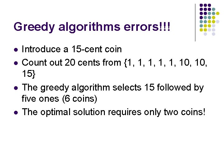
Greedy algorithms errors!!! l l Introduce a 15 -cent coin Count out 20 cents from {1, 1, 1, 10, 15} The greedy algorithm selects 15 followed by five ones (6 coins) The optimal solution requires only two coins!

Example: 0/1 knapsack problem l l l We are given a set of n items from which we are to select some number of items to be carried in a knapsack. Each item has both a weight and a profit. The objective is to chose the set of items that fits in the knapsack and maximizes the profit.

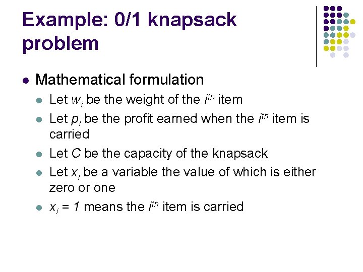
Example: 0/1 knapsack problem l Mathematical formulation l l l Let wi be the weight of the ith item Let pi be the profit earned when the ith item is carried Let C be the capacity of the knapsack Let xi be a variable the value of which is either zero or one xi = 1 means the ith item is carried

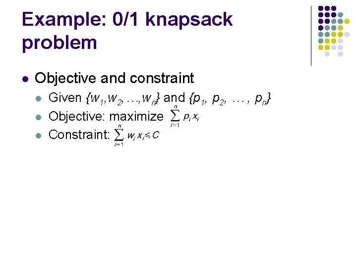
Example: 0/1 knapsack problem l Objective and constraint l l l Given {w 1, w 2, …, wn} and {p 1, p 2, … , pn} Objective: maximize Constraint:

Greedy possibilities l l l Greedy by Profit At each step select from the remaining items the one with the highest profit (provided the capacity of the knapsack is not exceeded). Greedy by Weight At each step select from the remaining items the one with the least weight (provided the capacity of the knapsack is not exceeded). Greedy by Profit Density At each step select from the remaining items the one with the largest profit density, pi/wi (provided the capacity of the knapsack is not exceeded).

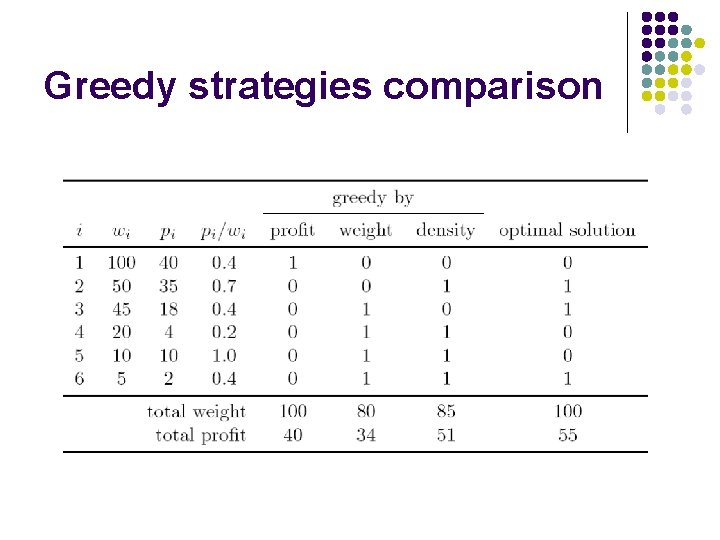
Greedy strategies comparison

Backtracking algorithms l l l View the problem as a sequence of decisions Systematically considers all possible outcomes for each decision Backtracking algorithms are like the brute-force algorithms However, they are distinguished by the way in which the space of possible solutions is explored Sometimes a backtracking algorithm can detect that an exhaustive search is not needed

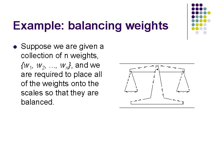
Example: balancing weights l Suppose we are given a collection of n weights, {w 1, w 2, . . . , wn}, and we are required to place all of the weights onto the scales so that they are balanced.

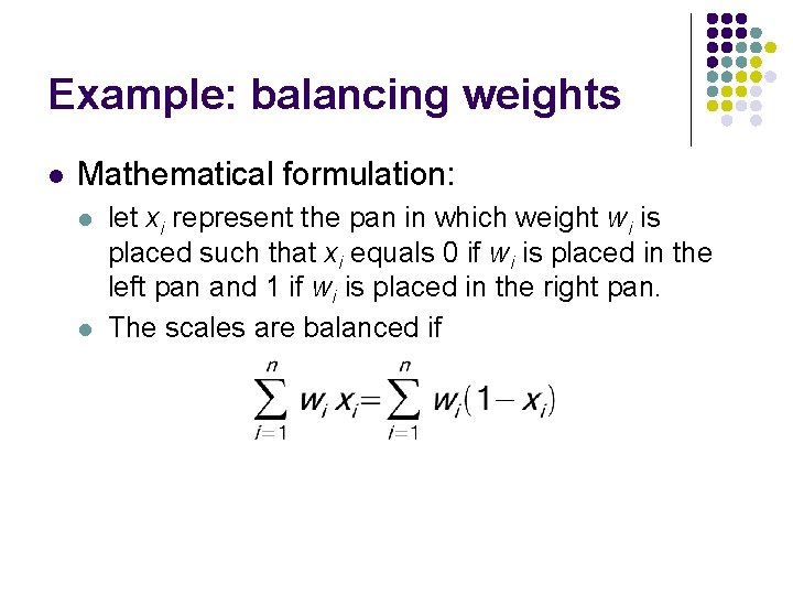
Example: balancing weights l Mathematical formulation: l l let xi represent the pan in which weight wi is placed such that xi equals 0 if wi is placed in the left pan and 1 if wi is placed in the right pan. The scales are balanced if

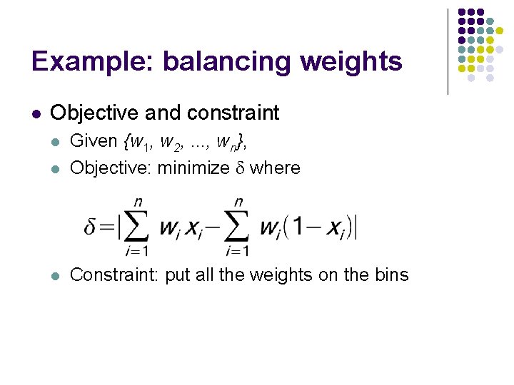
Example: balancing weights l Objective and constraint l Given {w 1, w 2, . . . , wn}, Objective: minimize where l Constraint: put all the weights on the bins l

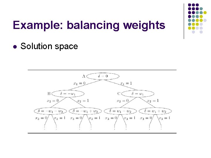
Example: balancing weights l Solution space

Example: balancing weights l l l In this case the solution space is a tree Each node represents a partial solution At each node measures the diference between the sum of the weights in each pan The solution tree has depth n and 2 n leaves The optimal solution is the leaf with the smallest

Backtracking solution l l l Visits all the nodes in the solution space Does a tree traversal! Possible traversals: l l Depth - first Breadth - first

Branch-and-bounds l Sometimes we can tell that a particular branch will not lead to an optimal solution: l l l the partial solution may already be infeasible already have another solution that is guaranteed to be better than any descendant of the given solution Prune the solution tree!

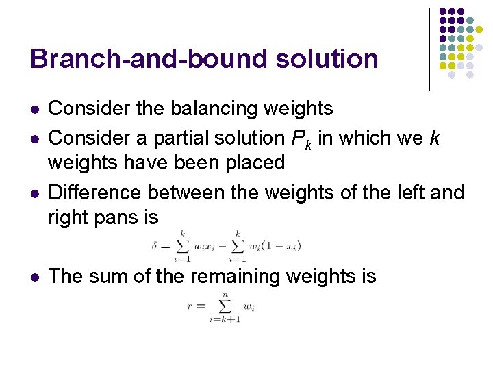
Branch-and-bound solution l l Consider the balancing weights Consider a partial solution Pk in which we k weights have been placed Difference between the weights of the left and right pans is The sum of the remaining weights is

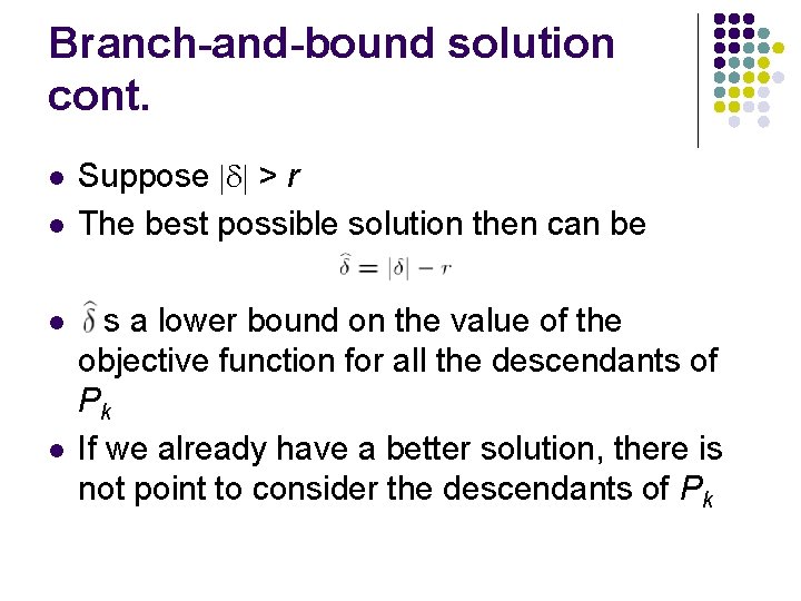
Branch-and-bound solution cont. l l Suppose > r The best possible solution then can be is a lower bound on the value of the objective function for all the descendants of Pk If we already have a better solution, there is not point to consider the descendants of Pk

Example: 0/1 knapsack again l l l Consider the previous 0/1 knapsack example A partial solution Sk is a solution where the first k items have been used If Sk is not feasible, than every other solution containing Sk is also infeasible. If Sk is feasible, than the total profit of any solution containing Sk is Just for comparison, a problem with 6 items has 64 possible solutions in a solution space of 127. If using breath or depth first solvers, they visit all the nodes and find all the solutions. If pruning is used, a possible solver visits only 67 nodes and finds 27 solution

Top-down strategies l Divide-and-conquer l l l To solve a problem, subdivide it into one or more sub problems each of which is similar to the given problem Solve each of the sub problems independently Combine the solutions to the sub problems to obtain a solution to the original problem Often implemented using recursion Sub problems are not overllaping

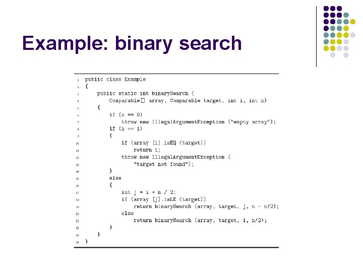
Example: binary search

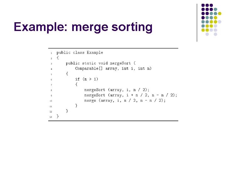
Example: merge sorting

Bottom-up strategies l Dynamic programming l l l To solve a given problem a series of sub problems is solved The series is devised so that each subsequent solution is obtained by combining two or more sub problems that have already been solved All intermediate solutions are kept in a table to prevent unnecessary repetition

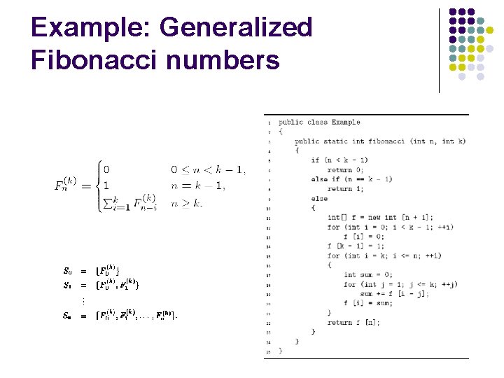
Example: Generalized Fibonacci numbers

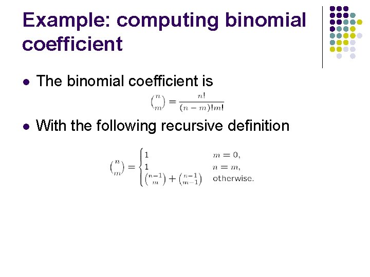
Example: computing binomial coefficient l The binomial coefficient is l With the following recursive definition

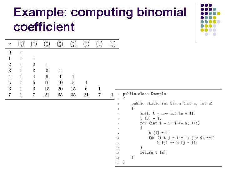
Example: computing binomial coefficient

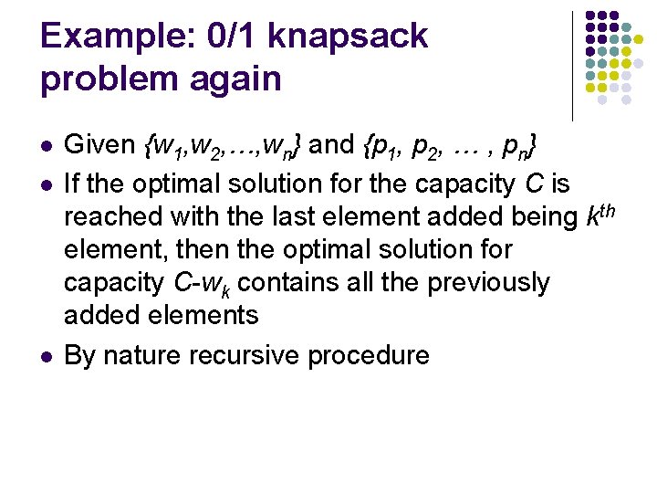
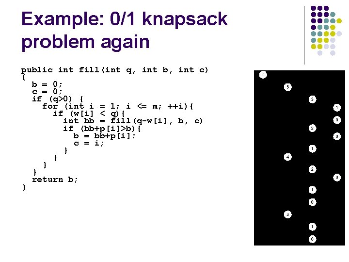
Example: 0/1 knapsack problem again l l l Given {w 1, w 2, …, wn} and {p 1, p 2, … , pn} If the optimal solution for the capacity C is reached with the last element added being kth element, then the optimal solution for capacity C-wk contains all the previously added elements By nature recursive procedure

Example: 0/1 knapsack problem again public int fill(int q, int b, int c) { b = 0; c = 0; if (q>0) { for (int i = 1; i <= m; ++i){ if (w[i] < q){ int bb = fill(q-w[i], b, c) if (bb+p[i]>b){ b = bb+p[i]; c = i; } } return b; }

Dynamic programming solution public void fill() { b[0] = 0; c[0] = 0; for (int q = 1; q <= n; ++q) { b[q] = 0; c[q] = 0; for (int i = 1; i <= m; ++i){ if (w[i] < q){ if ((b[q-w[i]]+p[i])>b[q]){ b[q] = b[q-w[i]]+p[i]; c[q] = i; } } }

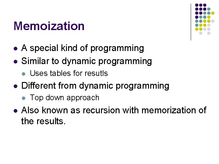
Memoization l l A special kind of programming Similar to dynamic programming l l Different from dynamic programming l l Uses tables for resutls Top down approach Also known as recursion with memorization of the results.

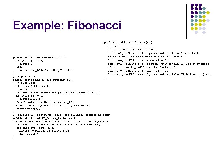
Example: Fibonacci public static void main() { int z; // this will be the slowest for (z=1; z<MAX; z++) System. out. writeln(Non_DP(z)); // this will be much faster than the first for (z=0; z<MAX; z++) memo[z] = 0; for (z=1; z<MAX; z++) System. out. writeln(DP_Top_Down(z)); /* this normally will be the fastest */ for (z=0; z<MAX; z++) memo[z] = 0; for (z=1; z<MAX; z++) System. out. writeln(DP_Bottom_Up(z)); } public static int Non_DP(int n) { if (n==1 || n==2) return 1; else return Non_DP(n-1) + Non_DP(n-2); } // top down DP public static int DP_Top_Down(int n) { // base case if (n == 1 || n == 2) return 1; // immediately return the previously computed result if (memo[n] != 0) return memo[n]; // otherwise, do the same as Non_DP memo[n] = DP_Top_Down(n-1) + DP_Top_Down(n-2); return memo[n]; } // fastest DP, bottom up, store the previous results in array public static int DP_Bottom_Up(int n) { memo[1] = memo[2] = 1; // default values for DP algorithm // from 3 to n (we already know that fib(1) and fib(2) = 1 for (int i=3; i<=n; i++) memo[i] = memo[i-1] + memo[i-2]; return memo[n]; }

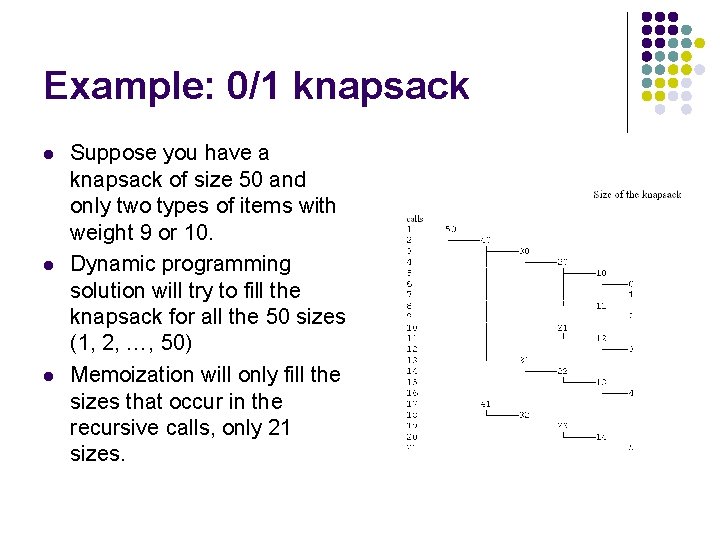
Example: 0/1 knapsack l l l Suppose you have a knapsack of size 50 and only two types of items with weight 9 or 10. Dynamic programming solution will try to fill the knapsack for all the 50 sizes (1, 2, …, 50) Memoization will only fill the sizes that occur in the recursive calls, only 21 sizes.

Reference l Preiss, ch. 14