Algorithmic Game Theory Uri Feige Robi Krauthgamer Moni

Algorithmic Game Theory Uri Feige Robi Krauthgamer Moni Naor Lecture 11: Combinatorial Auctions Lecturer: Moni Naor

Announcements • Course resumes to 1400: -16: 00

The setting • Set of alternatives A – Who wins the auction – Which path is chosen – Who is matched to whom • Each participant: a value function vi: A R • Can pay participants: valuation of choice a with payment pi is vi(a)+pi Quasi linear preferences

Mechanism Design • Mechanisms • Recall: We want to implement a social choice function – Need to know agents’ preferences – They may not reveal them to us truthfully • Example: – One item to allocate: • Want to give it to the participant who values it the most – If we just ask participants to tell us their preferences: may lie • Can use payments result is also a payment vector p=(p 1, p 2, … pn)

The Revelation Principle Theorem: if there exists an arbitrary mechanism implementing a social choice function f in dominant strategies, then there exists an incentive compatible mechanism that implements f The payments of the players in the incentive compatible mechanism are identical to those obtained at equilibrium in the original mechanism Proof: by simulation

Direct Characterization A mechanism is incentive compatible iff the following hold for all i and all vi • The payment pi does not depend on vi but only on the alternative chosen f(vi, v-i) – the payment of alternative a is pa • The mechanism optimizes for each player: f(vi, v-i) 2 argmaxa (vi(a)-pa)

Expected Revenues Theorem [Revenue Equivalence]: under very general conditions, every two Bayesian Nash implementations of the same social choice function if for some player and some type they have the same expected payment then – All types have the same expected payment to the player – If all player have the same expected payment: the expected revenues are the same Not true when there are reservation prices!

Range Voting • Each voter ranks the candidates in a certain range (say 0 -99) • The votes for all candidates are summed up and the one with highest total score wins Can be considered as a generalization of approval voting from the range 0 -1 No incentive for voter to rate a candidate lower than a candidate they like less.

• Vickrey Clarke Grove Mechanism f(v 1, v 2, … vn) maximizes i vi(a) over A – Maximizes welfare • There are functions h 1, h 2, … hn where hi: V 1 V 2 … Vn R does not depend on vi Depends only on chosen we have that: alternative pi(v 1, v 2, … vn) = hi(v-i) - j i vj(f(v 1, v 2, … vn)) Does not depend on vi Clark Pivot rule: Choosing hi(v-i) = maxb 2 A j i vj(b) Payment of i when a=f(v 1, v 2, …, vn): pwelfare vj(b)welfare - j(of iothers) vj(a) Social i(v 1, vwhen 2, … vn) = maxb 2 A j i. Social he does not when he participates

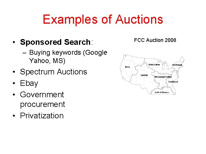
Examples of Auctions • Sponsored Search: – Buying keywords (Google, Yahoo, MS) • Spectrum Auctions • Ebay • Government procurement • Privatization FCC Auction 2008

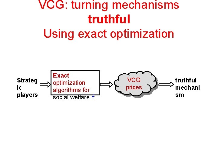
VCG: turning mechanisms truthful Using exact optimization Strateg ic players Exact optimization algorithms for social welfare f VCG prices truthful mechani sm

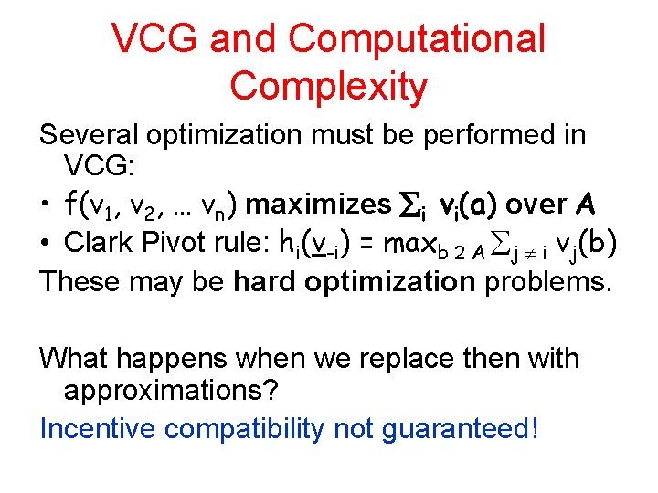
VCG and Computational Complexity Several optimization must be performed in VCG: • f(v 1, v 2, … vn) maximizes i vi(a) over A • Clark Pivot rule: hi(v-i) = maxb 2 A j i vj(b) These may be hard optimization problems. What happens when we replace then with approximations? Incentive compatibility not guaranteed!

Combinatorial Auctions • Set M of m indivisible items • Set N of n bidders • Preferences are on subsets S µ M – bundles – of items • Valuation function vi: 2 M R – vi(S) - value bidder i receives on bundle S • Must satisfy: monotonicity: v(s) · v(T) for S µ T • Normalized: v( ) = 0 Allocation: subsets S 1, S 2, … Sn where Si Å Sj = for i≠j Social welfare of allocation: n v (S )

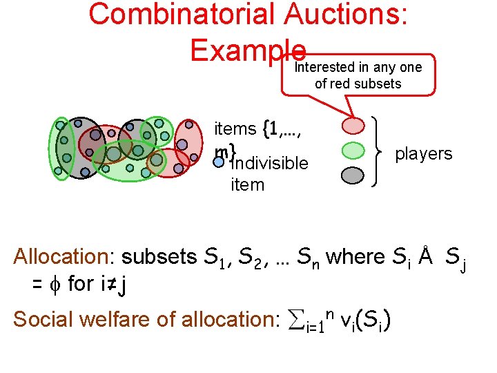
Combinatorial Auctions: Example. Interested in any one of red subsets items {1, …, m} indivisible item players Allocation: subsets S 1, S 2, … Sn where Si Å Sj = for i≠j Social welfare of allocation: i=1 n vi(Si)

Issues • Computational Complexity of finding the allocation maximizing the social welfare • Representation and communication of the valuation functions vi – May be large since defined for every subset • How to analyze the strategy of the bidder in light of the obstacles

Today • Complexity of Approximation – Tight bounds for the single minded bidder • Connection with communication complexity • Demand queries and the relaxed LP formulation

Single Minded Auctions A valuation v is single minded if there is a bundle of items S* and value v* 2 R such that – v(S) = v* if S* µ S – v(S) = 0 for all other S • Very simple to represent: (Si*, vi* ) Allocation problem for single minded bidders: • Given {(Si*, vi* )}i for bidders i=1. . n • Find a subset W of winning bids such that Si* Å Sj* = with maximum social welfare j 2 W vj*

Single Minded Auctions Example Allocation problem for single minded bidders: • Given {(Si*, vi* )}i for bidders i=1. . n • Find a subset W of winning bids such that Si* Å Sj* = with maximum social welfare j 2 W vj* Example: communication links in a tree • bidders want a path between some two nodes in the tree – Since there is only one path between any pair of nodes, the bidders are single-minded Bidder i wants to connect si to ti – Items = edges of tree – Si* = {set of edges connecting (si, ti) – v i* = 1

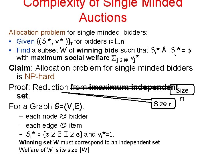
Complexity of Single Minded Auctions Allocation problem for single minded bidders: • Given {(Si*, vi* )}I for bidders i=1. . n • Find a subset W of winning bids such that Si* Å Sj* = with maximum social welfare j 2 W vj* Claim: Allocation problem for single minded bidders is NP-hard Proof: Reduction from imaximum independent. Size set. m Size n For a Graph G=(V, E): – each node bidder – each edge item – Si* = {e 2 E|I 2 e} and vi*=1. Winning set W must correspond to an independent set Welfare of W is its size |W|

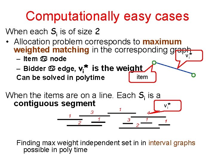
Computationally easy cases When each Si is of size 2 • Allocation problem corresponds to maximum weighted matching in the corresponding graph vi * – Item node – Bidder edge, vi* is the weight item Can be solved in polytime When the items are on a line. Each Si is a contiguous segment vi * Finding max weight independent set in in interval graphs possible in poly time

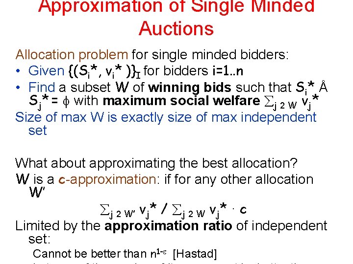
Approximation of Single Minded Auctions Allocation problem for single minded bidders: • Given {(Si*, vi* )}I for bidders i=1. . n • Find a subset W of winning bids such that Si* Å Sj* = with maximum social welfare j 2 W vj* Size of max W is exactly size of max independent set What about approximating the best allocation? W is a c-approximation: if for any other allocation W’ j 2 W’ vj* / j 2 W vj* · c Limited by the approximation ratio of independent set: Cannot be better than n 1 - [Hastad]

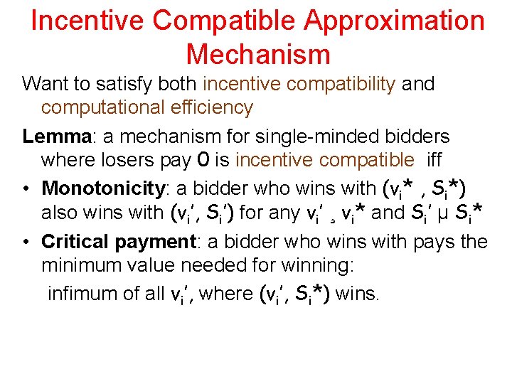
Incentive Compatible Approximation Mechanism Want to satisfy both incentive compatibility and computational efficiency Lemma: a mechanism for single-minded bidders where losers pay 0 is incentive compatible iff • Monotonicity: a bidder who wins with (vi* , Si*) also wins with (vi’, Si’) for any vi’ ¸ vi* and Si’ µ Si* • Critical payment: a bidder who wins with pays the minimum value needed for winning: infimum of all vi’, where (vi’, Si*) wins.

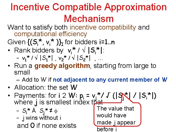
Incentive Compatible Approximation Mechanism Want to satisfy both incentive compatibility and computational efficiency Given {(Si*, vi* )}I for bidders i=1. . n • Rank bidders by vi* / √ |Si*|: – v 1* / √ |S 1*| ¸ v 2* / √ |S 2*| ¸ … • Run a greedy algorithm, starting from large to small – Add to W if not adjacent to any current member of W • Allocation: the set W • Payments: for i 2 W: pi = vj*/ √ (|Sj*| / |Si*|) where j is smallest index that The value that – S i* Å S j* ≠ – j wins without i and 0 if none exists would have made j appear before i

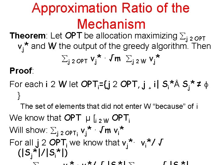
Approximation Ratio of the Mechanism Theorem: Let OPT be allocation maximizing j 2 OPT vj* and W the output of the greedy algorithm. Then j 2 OPT vj* · √m j 2 W vj* Proof: For each i 2 W let OPTi={j 2 OPT, j ¸ i| Si*Å Sj* ≠ } The set of elements that did not enter W “because” of i We know that OPT µ [i 2 W OPTi Will show: j 2 OPTi vj* · √m vi* For all j 2 OPTi we know that vj*· vi*/ √ (|Sj*|/|Si*|)

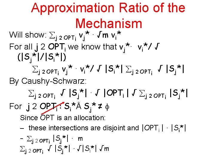
Approximation Ratio of the Mechanism Will show: j 2 OPTi vj* · √m vi* For all j 2 OPTi we know that vj*· vi*/ √ (|Sj*|/|Si*|) j 2 OPTi vj* · vi*/ √ |Si*| j 2 OPTi √ |Sj*| By Caushy-Schwarz: j 2 OPTi √ |Sj*| · √ |OPTi | √ j 2 OPTi |Sj*| For j 2 OPTi : Si*Å Sj* ≠ Since OPT is an allocation: – these intersections are disjoint and |OPTi | · |Si*| – j 2 OPTi |Sj*| · m j 2 OPTi √ |Sj*| · √|Si*| √m

Today • Complexity of Approximation – Tight bounds for the single minded bidder • Connection with communication complexity • Demand queries and the relaxed LP formulation

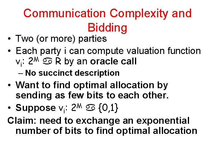
Communication Complexity and Bidding • Two (or more) parties • Each party i can compute valuation function vi: 2 M R by an oracle call – No succinct description • Want to find optimal allocation by sending as few bits to each other. • Suppose vi: 2 M {0, 1} Claim: need to exchange an exponential number of bits to find optimal allocation

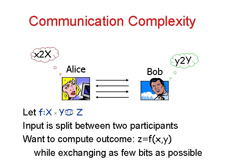
Communication Complexity x 2 X Alice Bob y 2 Y Let f: X x Y Z Input is split between two participants Want to compute outcome: z=f(x, y) while exchanging as few bits as possible

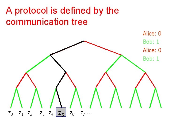
A protocol is defined by the communication tree Alice: 0 Bob: 1 z 0 z 1 z 2 z 3 z 4 zz 55 z 6 z 7. . .

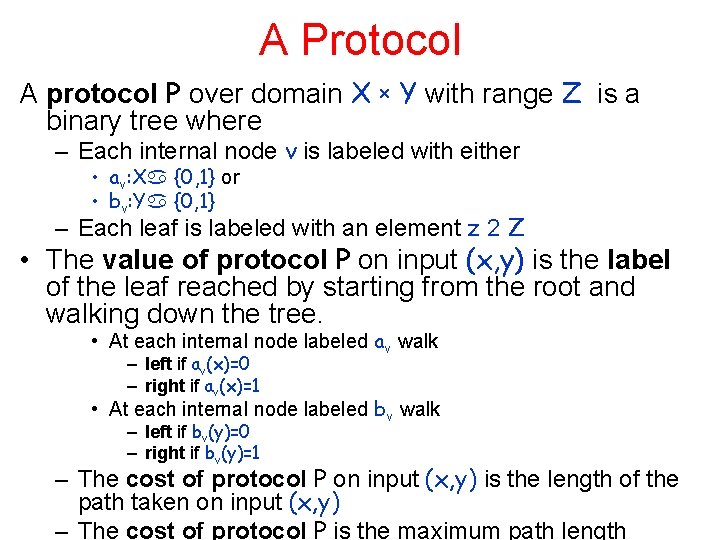
A Protocol A protocol P over domain X x Y with range Z is a binary tree where – Each internal node v is labeled with either • av: X {0, 1} or • bv: Y {0, 1} – Each leaf is labeled with an element z 2 Z • The value of protocol P on input (x, y) is the label of the leaf reached by starting from the root and walking down the tree. • At each internal node labeled av walk – left if av(x)=0 – right if av(x)=1 • At each internal node labeled bv walk – left if bv(y)=0 – right if bv(y)=1 – The cost of protocol P on input (x, y) is the length of the path taken on input (x, y) – The cost of protocol P is the maximum path length

Motivation for studying communication complexity • • • Originally for studying VLSI questions Connection with Turing Machines Data structures and the cell probe model Boolean circuit depth Combinatorial Auctions …

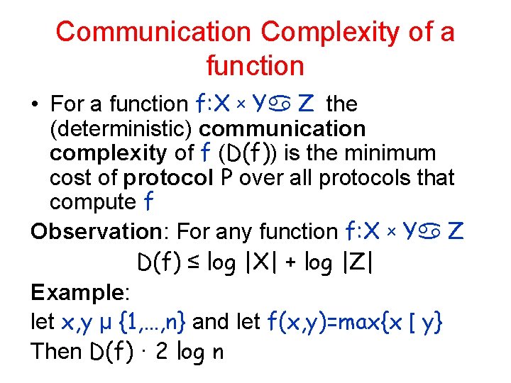
Communication Complexity of a function • For a function f: X x Y Z the (deterministic) communication complexity of f (D(f)) is the minimum cost of protocol P over all protocols that compute f Observation: For any function f: X x Y Z D(f) ≤ log |X| + log |Z| Example: let x, y µ {1, …, n} and let f(x, y)=max{x [ y} Then D(f) · 2 log n

Combinatorial Rectangles • A combinatorial rectangle in X x Y is a subset R µ X x Y such that R= A x B for some A µ X and B µ Y Proposition: R µ X x Y is a combinatorial rectangle iff (x 1, y 1) 2 R and (x 2, y 2) 2 R implies that (x 1, y 2) 2 R For Protocol P and node v let Rv be the set of inputs (x, y) reaching v Claim: For any protocol P and node v the set Rv is a combinatorial rectangle Claim: given the transcript of an exchange between Alice an Bob (but not x and y) possible to determine z=f(x, y)

Fooling Sets • For f: X x Y Z a subset R µ X x Y is f-monochromatic if f is fixed on R • Observation: any protocol P induces a partition of X x Y into f-monochromatic rectangles. – The number of rectangles is the number of leaves in P • A set Sµ X x Y is a fooling set for f if there exists a z 2 Z where – For every (x, y) 2 S, f(x, y)=z – For every distinct (x 1, y 1), (x 2, y 2) 2 S either • f(x 1, y 2)≠z or • f(x 2, y 1)≠z Property: no two elements of a fooling set S can be in the same monochromatic rectangle Lemma: if f has a fooling set of size t, then D(f) ≥ log 2 t

Examples Equality: Alice and Bob each hold x, y 2 {0, 1}n – want to decide whether x=y or not. • Fooling set for Equality S={(w, w)|w 2 {0, 1}n } Conclusion: D(Equality) ¸ n Disjointness: let x, y µ {1, …, n} and let – DISJ(x, y)=1 if |x y|¸ 1 and – DISJ(x, y)=0 otherwise • Fooling set for Disjointness S={(A, comp(A))|A µ {1, …, n} } Conclusion: D(DISJ) ¸ n

Bidding as a function • In bidding the parties are interested in finding a good allocation • Can be viewed as computing a relation • Can view the

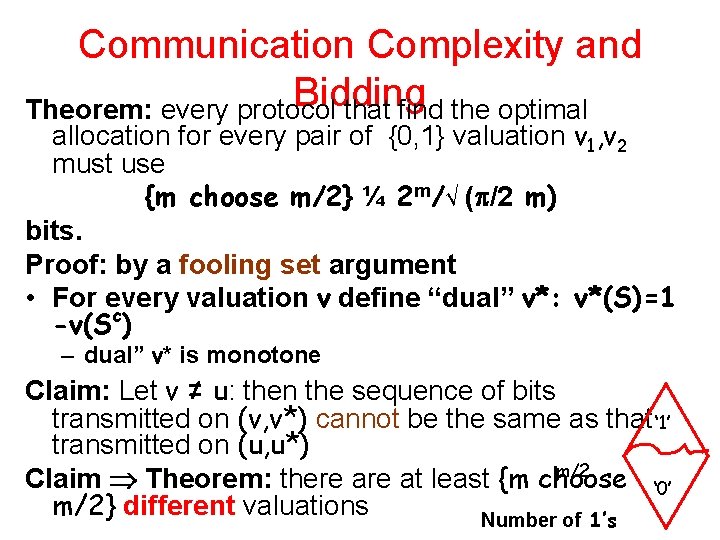
Communication Complexity and Bidding Theorem: every protocol that find the optimal allocation for every pair of {0, 1} valuation v 1, v 2 must use {m choose m/2} ¼ 2 m/√ ( /2 m) bits. Proof: by a fooling set argument • For every valuation v define “dual” v*: v*(S)=1 -v(Sc) – dual” v* is monotone Claim: Let v ≠ u: then the sequence of bits transmitted on (v, v*) cannot be the same as that ‘ 1’ transmitted on (u, u*) m/2 Claim Theorem: there at least {m choose ‘ 0’ m/2} different valuations Number of 1’s

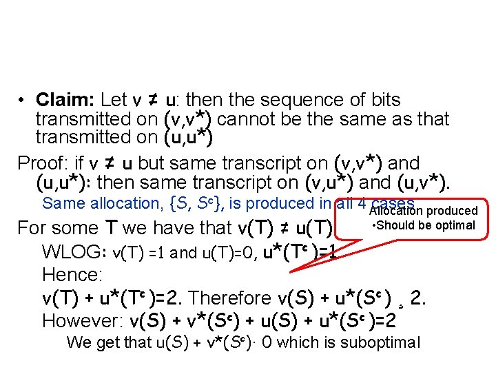
• Claim: Let v ≠ u: then the sequence of bits transmitted on (v, v*) cannot be the same as that transmitted on (u, u*) Proof: if v ≠ u but same transcript on (v, v*) and (u, u*): then same transcript on (v, u*) and (u, v*). Same allocation, {S, Sc}, is produced in all 4 Allocation cases produced • Should be optimal For some T we have that v(T) ≠ u(T). WLOG: v(T) =1 and u(T)=0, u*(Tc )=1. Hence: v(T) + u*(Tc )=2. Therefore v(S) + u*(Sc ) ¸ 2. However: v(S) + v*(Sc) + u(S) + u*(Sc )=2 We get that u(S) + v*(Sc)· 0 which is suboptimal

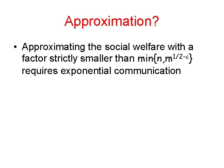
Approximation? • Approximating the social welfare with a factor strictly smaller than min{n, m 1/2 - } requires exponential communication

Today • Complexity of Approximation – Tight bounds for the single minded bidder • Connection with communication complexity • Demand queries and the relaxed LP formulation

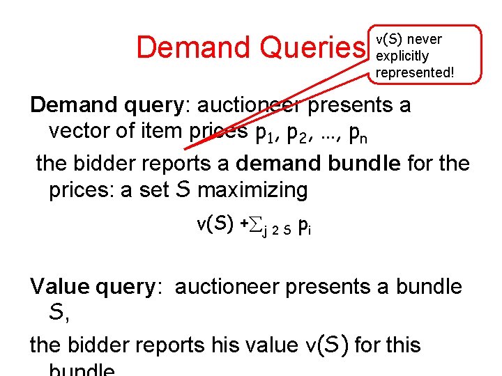
Demand Queries v(S) never explicitly represented! Demand query: auctioneer presents a vector of item prices p 1, p 2, …, pn the bidder reports a demand bundle for the prices: a set S maximizing v(S) + j 2 S pi Value query: auctioneer presents a bundle S, the bidder reports his value v(S) for this

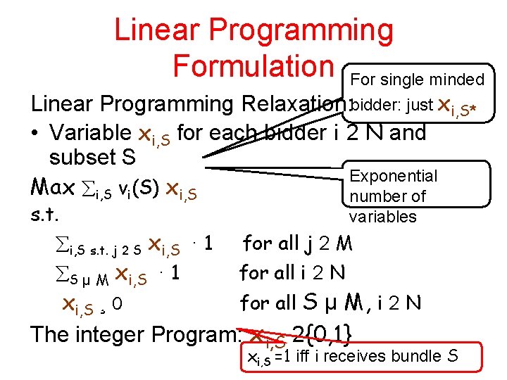
Linear Programming Formulation For single minded Linear Programming Relaxation: bidder: just xi, S* • Variable xi, S for each bidder i 2 N and subset S Exponential Max i, S vi(S) xi, S number of s. t. i, S s. t. j 2 S xi, S · 1 S µ M xi, S · 1 variables for all j 2 M for all i 2 N xi, S ¸ 0 for all S µ M, i 2 N The integer Program: xi, S 2{0, 1} xi, S =1 iff i receives bundle S

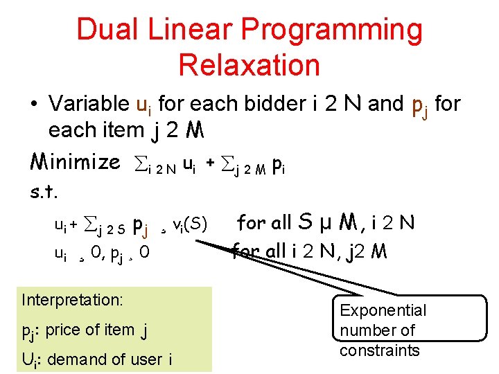
Dual Linear Programming Relaxation • Variable ui for each bidder i 2 N and pj for each item j 2 M Minimize i 2 N ui + j 2 M pi s. t. ui + j 2 S pj ¸ vi(S) ui ¸ 0, pj ¸ 0 Interpretation: pj: price of item j Ui: demand of user i for all S µ M, i 2 N for all i 2 N, j 2 M Exponential number of constraints

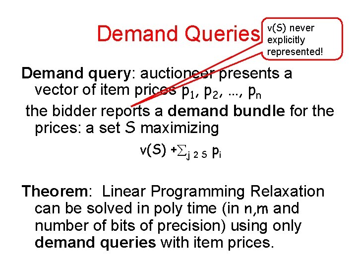
Demand Queries v(S) never explicitly represented! Demand query: auctioneer presents a vector of item prices p 1, p 2, …, pn the bidder reports a demand bundle for the prices: a set S maximizing v(S) + j 2 S pi Theorem: Linear Programming Relaxation can be solved in poly time (in n, m and number of bits of precision) using only demand queries with item prices.

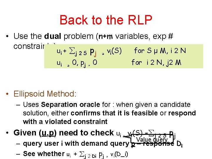
Back to the RLP • Use the dual problem (n+m variables, exp # constraints) u + p ¸ v (S) for S µ M, i 2 N i j 2 S j ui ¸ 0, pj ¸ 0 i for i 2 N, j 2 M • Ellipsoid Method: – Uses Separation oracle for : when given a candidate solution, either confirms that it is feasible or respond with a violated constraint • Given (u, p) need to check ui ¸ vi(S) - j 2 S pj Value query – query user i with demand query p – response Di – See whether ui + j 2 Di pj ¸ vi(D_i)

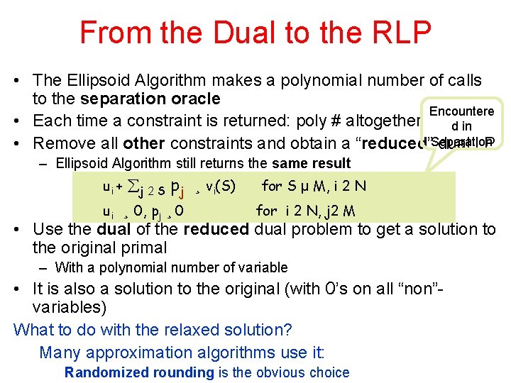
From the Dual to the RLP • The Ellipsoid Algorithm makes a polynomial number of calls to the separation oracle Encountere • Each time a constraint is returned: poly # altogether d in • Remove all other constraints and obtain a “reduced”Separation dual LP – Ellipsoid Algorithm still returns the same result j 2 S pj ¸ vi(S) for S µ M, i 2 N ui ¸ 0, pj ¸ 0 for i 2 N, j 2 M • Use the dual of the reduced dual problem to get a solution to the original primal ui + – With a polynomial number of variable • It is also a solution to the original (with 0’s on all “non”variables) What to do with the relaxed solution? Many approximation algorithms use it: Randomized rounding is the obvious choice