Algorithm Evaluation and Error Analysis class 7 Multiple

Algorithm Evaluation and Error Analysis class 7 Multiple View Geometry Comp 290 -089 Marc Pollefeys

Multiple View Geometry course schedule (subject to change) Jan. 7, 9 Intro & motivation Projective 2 D Geometry Jan. 14, 16 (no class) Projective 2 D Geometry Jan. 21, 23 Projective 3 D Geometry (no class) Jan. 28, 30 Parameter Estimation Feb. 4, 6 Algorithm Evaluation Camera Models Feb. 11, 13 Camera Calibration Single View Geometry Feb. 18, 20 Epipolar Geometry 3 D reconstruction Feb. 25, 27 Fund. Matrix Comp. Structure Comp. Planes & Homographies Trifocal Tensor Three View Reconstruction Multiple View Geometry Mar. 4, 6 Mar. 18, 20 Mar. 25, 27 Multiple. View Reconstruction Bundle adjustment Apr. 1, 3 Auto-Calibration Papers Apr. 8, 10 Dynamic Sf. M Papers Apr. 15, 17 Cheirality Papers Apr. 22, 24 Duality Project Demos

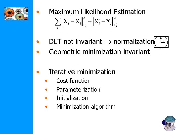
• Maximum Likelihood Estimation • • DLT not invariant normalization Geometric minimization invariant • Iterative minimization • • Cost function Parameterization Initialization Minimization algorithm

Automatic computation of H Objective Compute homography between two images Algorithm (i) Interest points: Compute interest points in each image (ii) Putative correspondences: Compute a set of interest point matches based on some similarity measure (iii) RANSAC robust estimation: Repeat for N samples (iv) (a) Select 4 correspondences and compute H (v) (b) Calculate the distance d for each putative match (vi) (c) Compute the number of inliers consistent with H (d <t) (vii) Choose H with most inliers (iv) Optimal estimation: re-estimate H from all inliers by minimizing ML cost function with Levenberg-Marquardt (v) Guided matching: Determine more matches using prediction by computed H

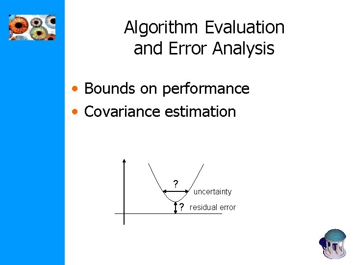
Algorithm Evaluation and Error Analysis • Bounds on performance • Covariance estimation ? uncertainty ? residual error

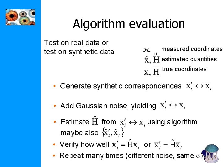
Algorithm evaluation Test on real data or test on synthetic data measured coordinates estimated quantities true coordinates • Generate synthetic correspondences • Add Gaussian noise, yielding • Estimate from maybe also using algorithm • Verify how well or • Repeat many times (different noise, same s)

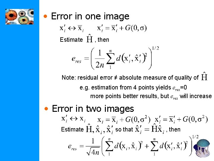
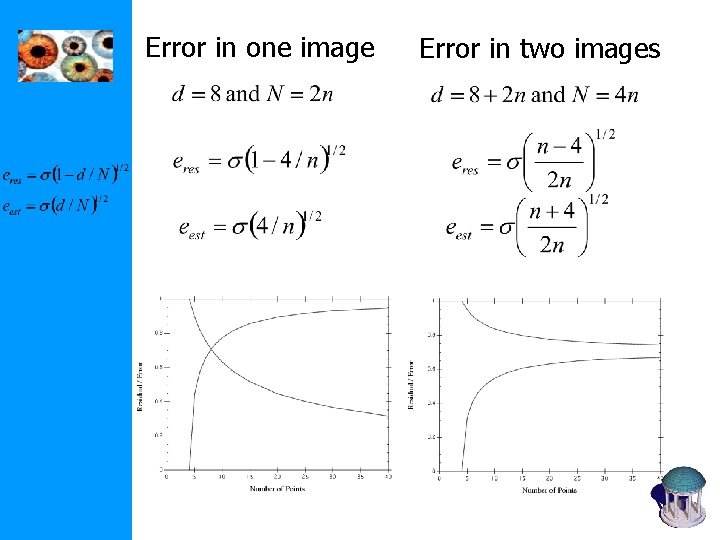
• Error in one image Estimate , then Note: residual error ≠ absolute measure of quality of e. g. estimation from 4 points yields eres=0 more points better results, but eres will increase • Error in two images Estimate so that , then

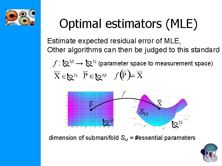
Optimal estimators (MLE) Estimate expected residual error of MLE, Other algorithms can then be judged to this standard f : M → N (parameter space to measurement space) N M f X P SM M N dimension of submanifold SM = #essential parameters

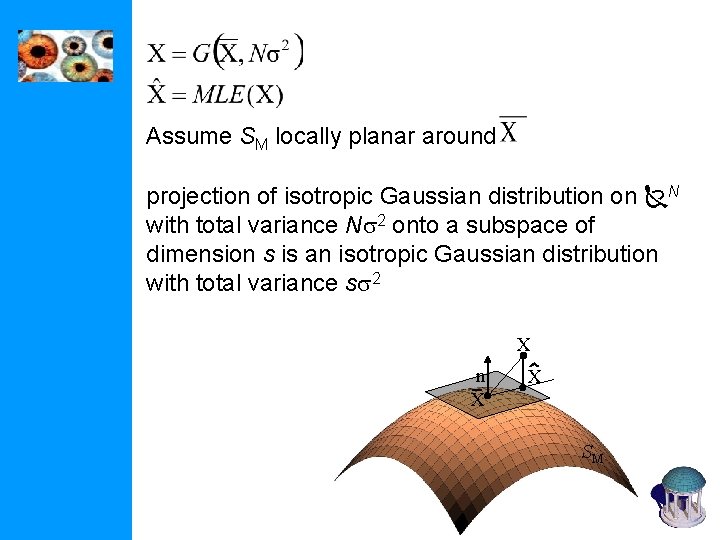
Assume SM locally planar around projection of isotropic Gaussian distribution on N with total variance Ns 2 onto a subspace of dimension s is an isotropic Gaussian distribution with total variance ss 2 X n X X SM

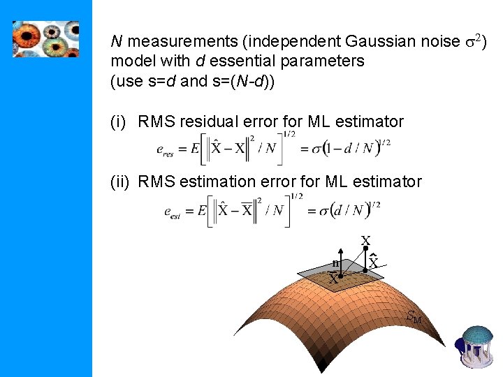
N measurements (independent Gaussian noise s 2) model with d essential parameters (use s=d and s=(N-d)) (i) RMS residual error for ML estimator (ii) RMS estimation error for ML estimator X n X X SM

Error in one image Error in two images

Covariance of estimated model • Previous question: how close is the error to smallest possible error? • Independent of point configuration • Real question: how close is estimated model to real model? • Dependent on point configuration (e. g. 4 points close to a line)

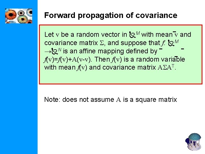
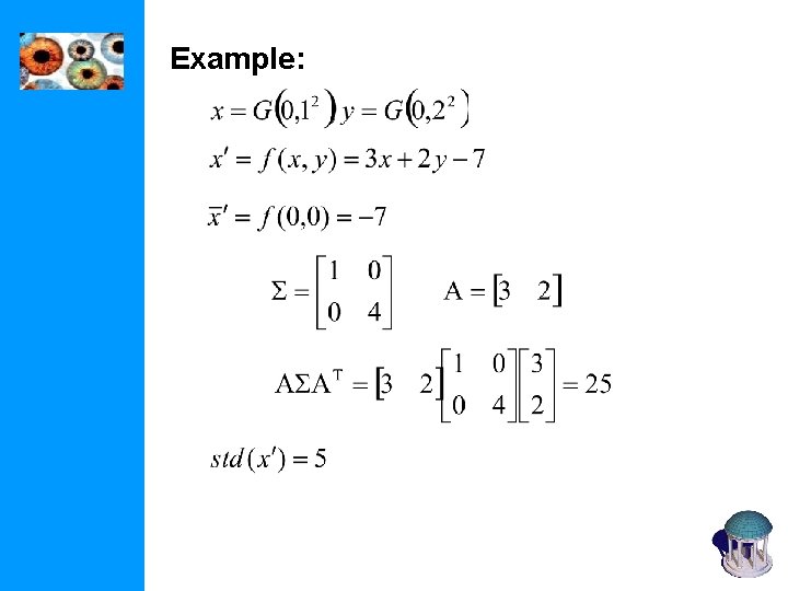
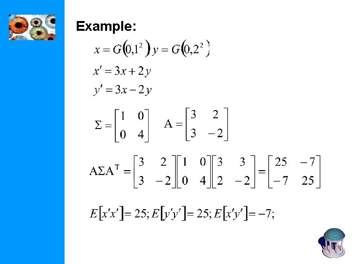
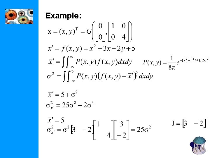
Forward propagation of covariance Let v be a random vector in M with mean v and covariance matrix S, and suppose that f: M → N is an affine mapping defined by f(v)=f(v)+A(v-v). Then f(v) is a random variable with mean f(v) and covariance matrix ASAT. Note: does not assume A is a square matrix

Example:

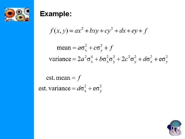
Example:

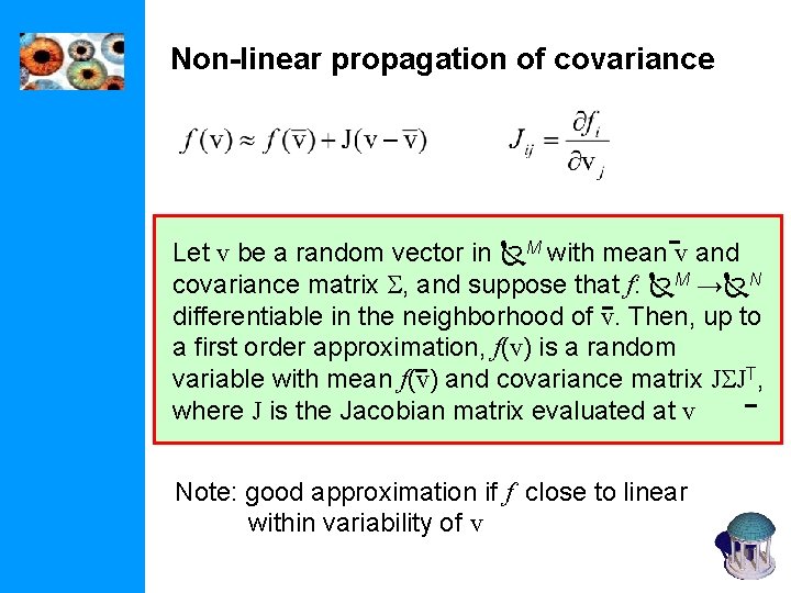
Non-linear propagation of covariance Let v be a random vector in M with mean v and covariance matrix S, and suppose that f: M → N differentiable in the neighborhood of v. Then, up to a first order approximation, f(v) is a random variable with mean f(v) and covariance matrix JSJT, where J is the Jacobian matrix evaluated at v Note: good approximation if f close to linear within variability of v

Example:

Example:

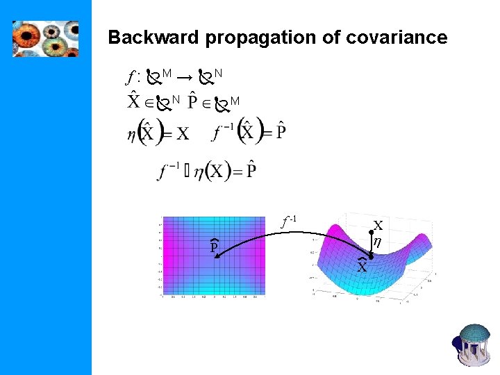
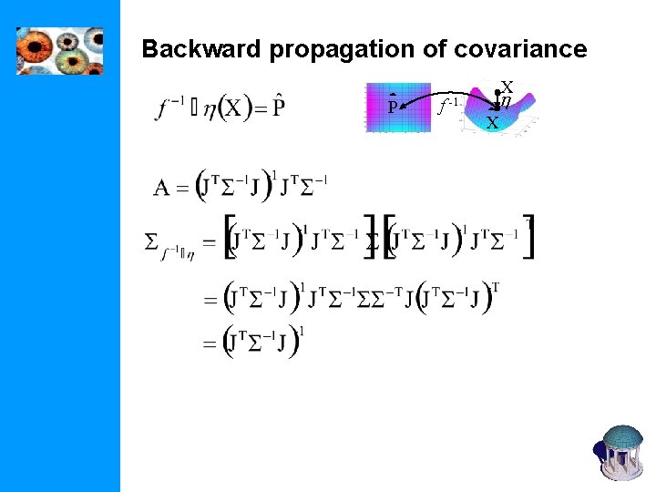
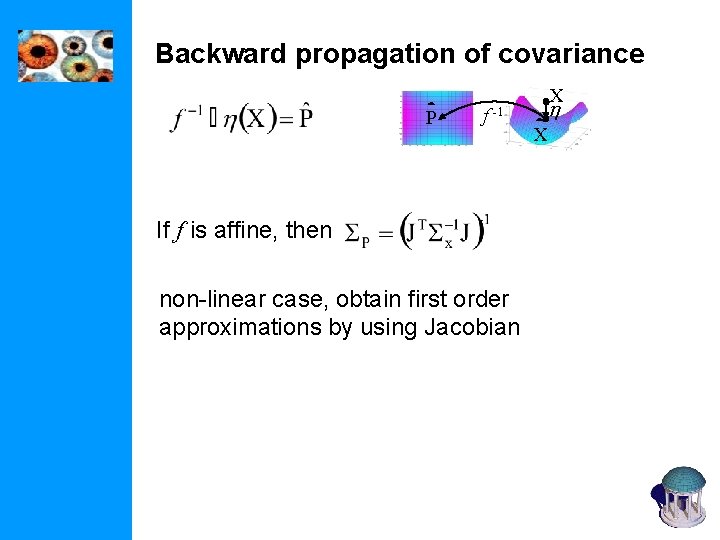
Backward propagation of covariance f : M → N N M f -1 X h P X

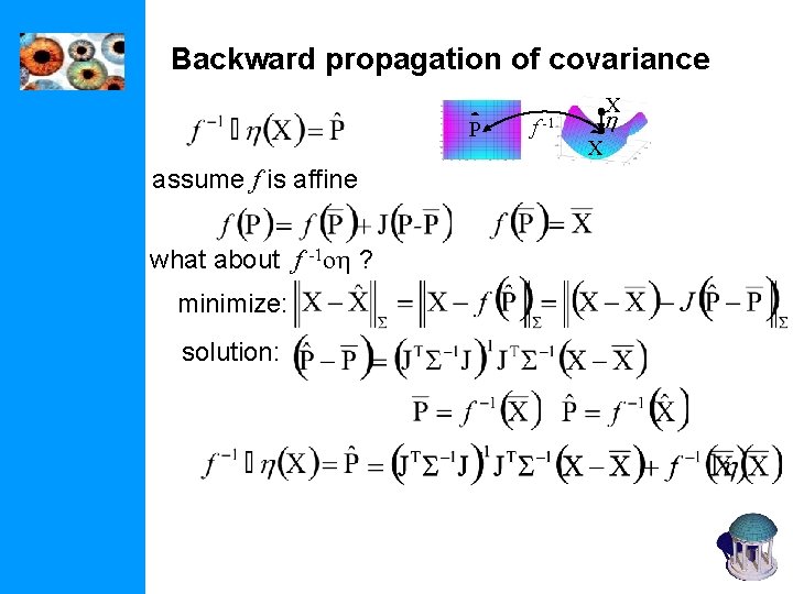
Backward propagation of covariance P assume f is affine what about f -1 oh ? minimize: solution: f X h -1 X

Backward propagation of covariance P f X h -1 X

Backward propagation of covariance P f X h -1 If f is affine, then non-linear case, obtain first order approximations by using Jacobian X

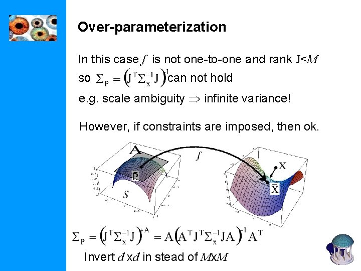
Over-parameterization In this case f is not one-to-one and rank J<M so can not hold e. g. scale ambiguity infinite variance! However, if constraints are imposed, then ok. Invert d xd in stead of Mx. M

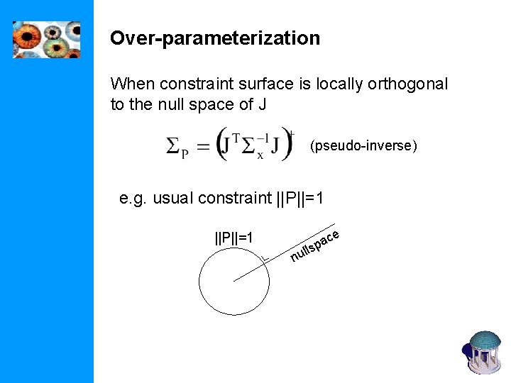
Over-parameterization When constraint surface is locally orthogonal to the null space of J (pseudo-inverse) e. g. usual constraint ||P||=1 lls nu e c pa

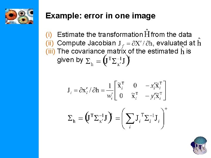
Example: error in one image (i) Estimate the transformation from the data (ii) Compute Jacobian , evaluated at (iii) The covariance matrix of the estimated is given by

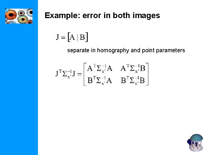
Example: error in both images separate in homography and point parameters

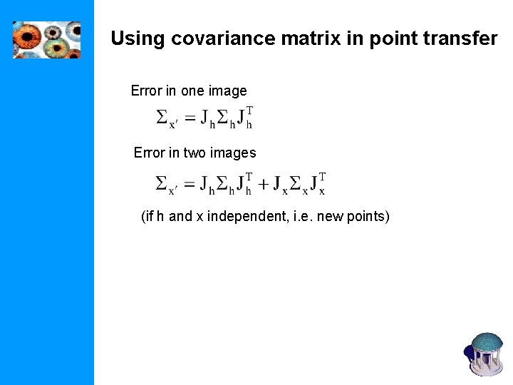
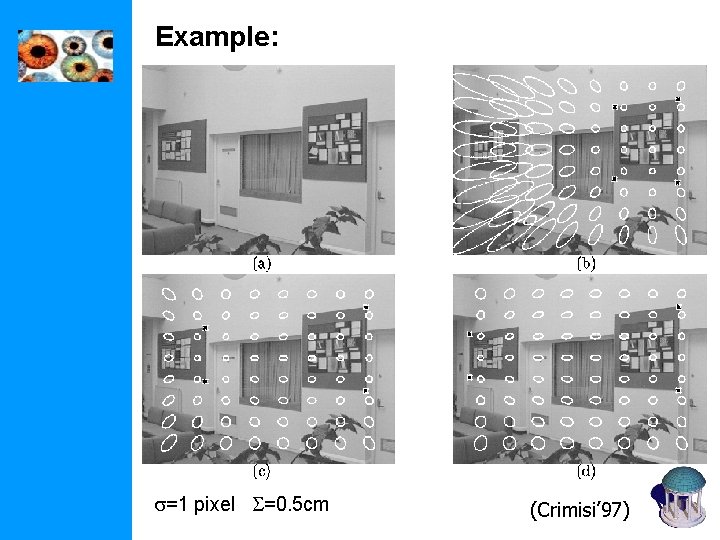
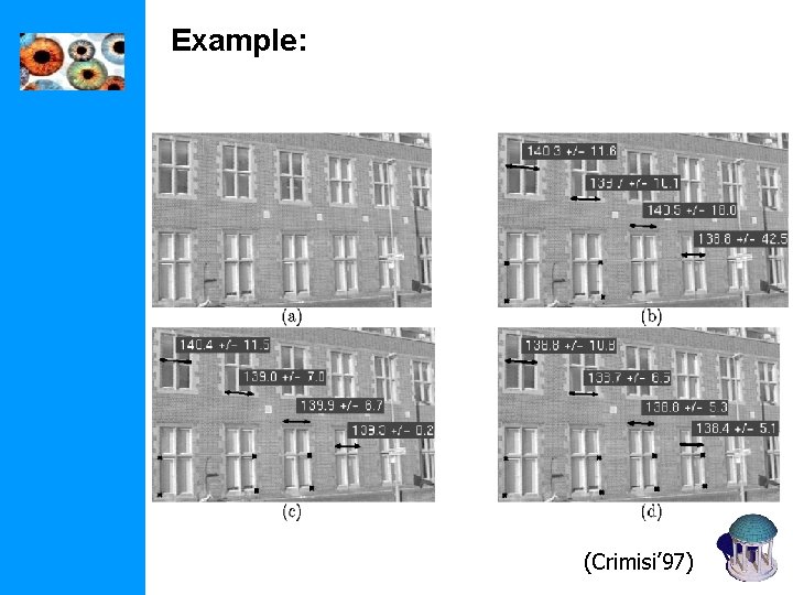
Using covariance matrix in point transfer Error in one image Error in two images (if h and x independent, i. e. new points)

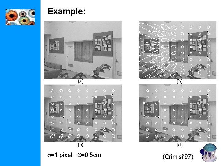
Example: s=1 pixel S=0. 5 cm (Crimisi’ 97)

Example: s=1 pixel S=0. 5 cm (Crimisi’ 97)

Example: (Crimisi’ 97)

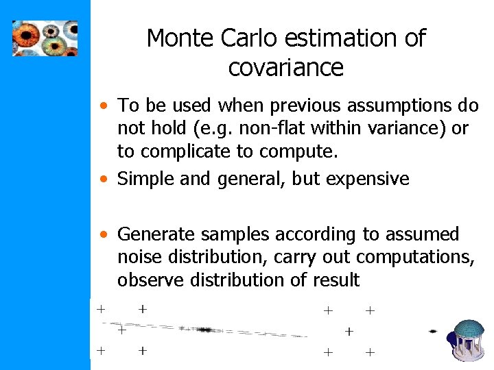
Monte Carlo estimation of covariance • To be used when previous assumptions do not hold (e. g. non-flat within variance) or to complicate to compute. • Simple and general, but expensive • Generate samples according to assumed noise distribution, carry out computations, observe distribution of result

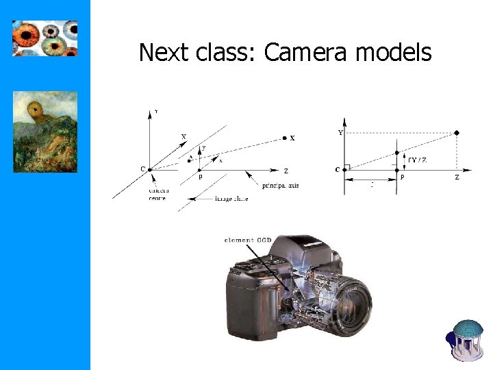
Next class: Camera models