Algorithm Design Techniques Greedy Method Knapsack Problem Job

Algorithm Design Techniques, Greedy Method – Knapsack Problem, Job Sequencing, Divide and Conquer Method – Quick Sort, Finding Maximum and Minimum, Dynamic programming- Matrix chain multiplication

Algorithm Design Techniques, • DESIGN TECHNIQUES Divide-and-Conquer. Prune-and-Search. Dynamic Programming. Greedy Algorithms.

Divide-and-Conquer. Essence of Divide and Conquer • Divide problem into several smaller sub problems – Normally, the sub problems are similar to the original • Conquer the sub problems by solving them recursively – Base case: solve small enough problems by brute force • Combine the solutions to get a solution to the sub problems – And finally a solution to the original problem • Divide and Conquer algorithms are normally recursive

Divide-and-Conquer -Quick Sort • Quick. Sort uses Divide-and-Conquer recursive algorithm. • To sort the values Divide and Conquer is one of the famous algorithmic techniques. • It works with the philosophy that divide the whole problem into smaller manageable chunks of sub problems and work out these small sub problems there by combining the intermediate partial solutions. • There are many famous examples which use the Divide and Conquer strategy, for example Binary search, Merge sort, Insertion sort, Quick sort etc. ,

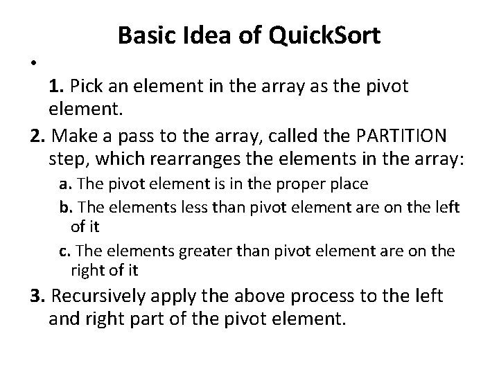
• Basic Idea of Quick. Sort 1. Pick an element in the array as the pivot element. 2. Make a pass to the array, called the PARTITION step, which rearranges the elements in the array: a. The pivot element is in the proper place b. The elements less than pivot element are on the left of it c. The elements greater than pivot element are on the right of it 3. Recursively apply the above process to the left and right part of the pivot element.

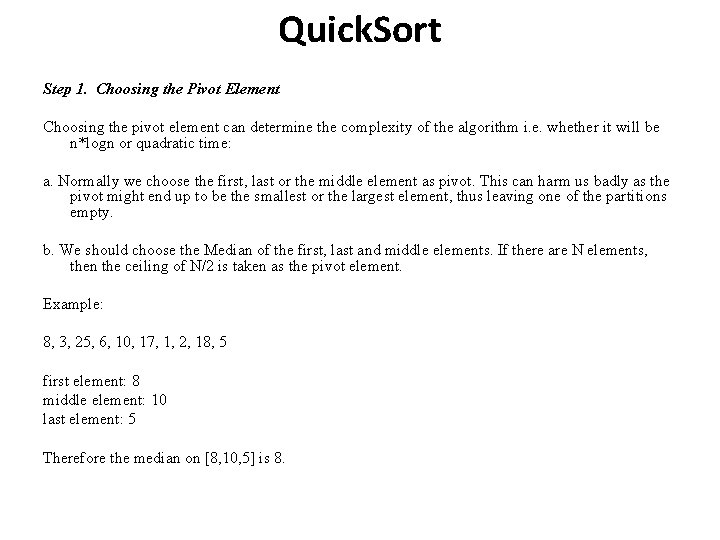
Quick. Sort Step 1. Choosing the Pivot Element Choosing the pivot element can determine the complexity of the algorithm i. e. whether it will be n*logn or quadratic time: a. Normally we choose the first, last or the middle element as pivot. This can harm us badly as the pivot might end up to be the smallest or the largest element, thus leaving one of the partitions empty. b. We should choose the Median of the first, last and middle elements. If there are N elements, then the ceiling of N/2 is taken as the pivot element. Example: 8, 3, 25, 6, 10, 17, 1, 2, 18, 5 first element: 8 middle element: 10 last element: 5 Therefore the median on [8, 10, 5] is 8.

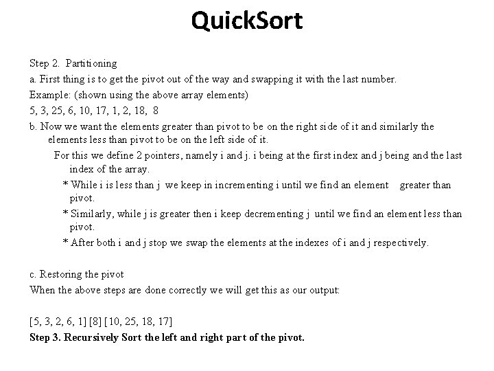
Quick. Sort Step 2. Partitioning a. First thing is to get the pivot out of the way and swapping it with the last number. Example: (shown using the above array elements) 5, 3, 25, 6, 10, 17, 1, 2, 18, 8 b. Now we want the elements greater than pivot to be on the right side of it and similarly the elements less than pivot to be on the left side of it. For this we define 2 pointers, namely i and j. i being at the first index and j being and the last index of the array. * While i is less than j we keep in incrementing i until we find an element greater than pivot. * Similarly, while j is greater then i keep decrementing j until we find an element less than pivot. * After both i and j stop we swap the elements at the indexes of i and j respectively. c. Restoring the pivot When the above steps are done correctly we will get this as our output: [5, 3, 2, 6, 1] [8] [10, 25, 18, 17] Step 3. Recursively Sort the left and right part of the pivot.

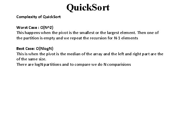
Quick. Sort Complexity of Quick. Sort Worst Case : O(N^2) This happens when the pivot is the smallest or the largest element. Then one of the partition is empty and we repeat the recursion for N-1 elements Best Case: O(Nlog. N) This is when the pivot is the median of the array and the left and right part are the of the same size. There are log. N partitions and to compare we do N comparisions

Analysis of Quick Sort • How is it that quick sort's worst-case and average -case running times differ? • Let's start by looking at the worst-case running time. – Suppose that we're really unlucky and the partition sizes are really unbalanced. In particular, suppose that the pivot chosen by the partition function is always either the smallest or the largest element in the nnelement subarray. Then one of the partitions will contain no elements and the other partition will contain n-1 n− 1 elements—all but the pivot. So the recursive calls will be on sub arrays of sizes 0 and n 1 n− 1.

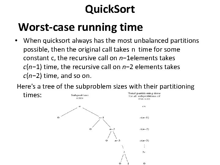
Quick. Sort Worst-case running time • When quicksort always has the most unbalanced partitions possible, then the original call takes n time for some constant c, the recursive call on n− 1 elements takes c(n− 1) time, the recursive call on n− 2 elements takes c(n− 2) time, and so on. Here's a tree of the subproblem sizes with their partitioning times:

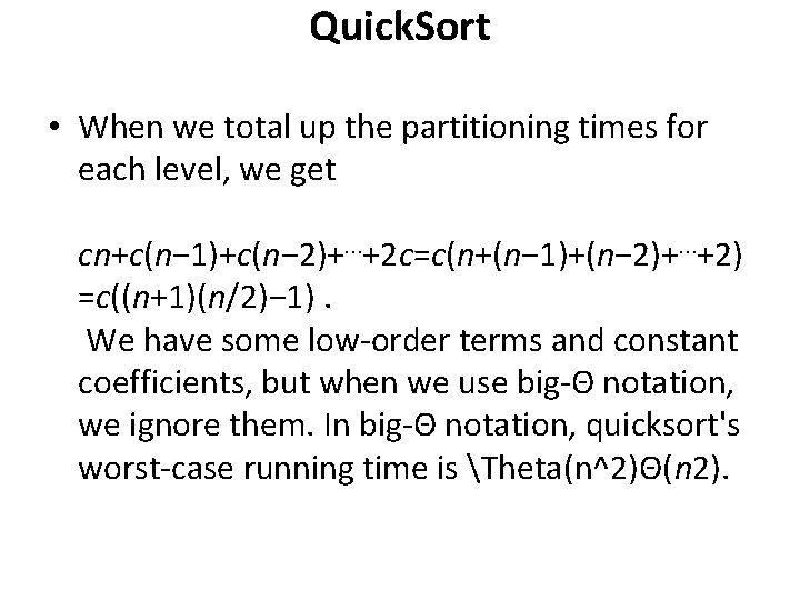
Quick. Sort • When we total up the partitioning times for each level, we get cn+c(n− 1)+c(n− 2)+⋯+2 c=c(n+(n− 1)+(n− 2)+⋯+2) =c((n+1)(n/2)− 1). We have some low-order terms and constant coefficients, but when we use big-Θ notation, we ignore them. In big-Θ notation, quicksort's worst-case running time is Theta(n^2)Θ(n 2).

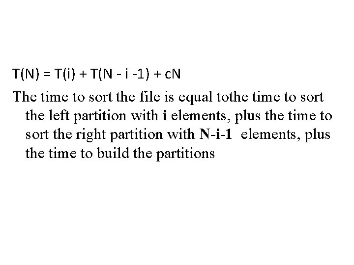
T(N) = T(i) + T(N - i -1) + c. N The time to sort the file is equal tothe time to sort the left partition with i elements, plus the time to sort the right partition with N-i-1 elements, plus the time to build the partitions

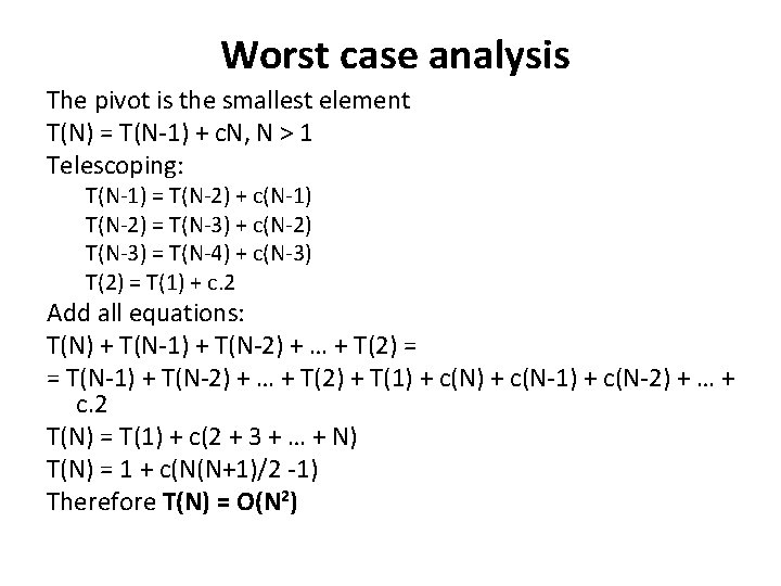
Worst case analysis The pivot is the smallest element T(N) = T(N-1) + c. N, N > 1 Telescoping: T(N-1) = T(N-2) + c(N-1) T(N-2) = T(N-3) + c(N-2) T(N-3) = T(N-4) + c(N-3) T(2) = T(1) + c. 2 Add all equations: T(N) + T(N-1) + T(N-2) + … + T(2) = = T(N-1) + T(N-2) + … + T(2) + T(1) + c(N-1) + c(N-2) + … + c. 2 T(N) = T(1) + c(2 + 3 + … + N) T(N) = 1 + c(N(N+1)/2 -1) Therefore T(N) = O(N 2)

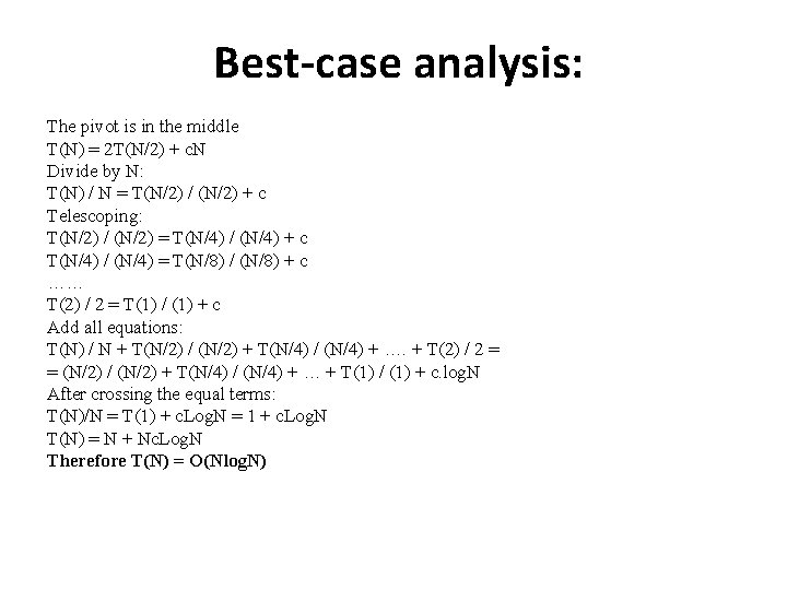
Best-case analysis: The pivot is in the middle T(N) = 2 T(N/2) + c. N Divide by N: T(N) / N = T(N/2) / (N/2) + c Telescoping: T(N/2) / (N/2) = T(N/4) / (N/4) + c T(N/4) / (N/4) = T(N/8) / (N/8) + c …… T(2) / 2 = T(1) / (1) + c Add all equations: T(N) / N + T(N/2) / (N/2) + T(N/4) / (N/4) + …. + T(2) / 2 = = (N/2) / (N/2) + T(N/4) / (N/4) + … + T(1) / (1) + c. log. N After crossing the equal terms: T(N)/N = T(1) + c. Log. N = 1 + c. Log. N T(N) = N + Nc. Log. N Therefore T(N) = O(Nlog. N)

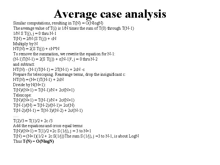
Average case analysis Similar computations, resulting in T(N) = O(Nlog. N) The average value of T(i) is 1/N times the sum of T(0) through T(N-1) 1/N S T(j), j = 0 thru N-1 T(N) = 2/N (S T(j)) + c. N Multiply by N NT(N) = 2(S T(j)) + c. N*N To remove the summation, we rewrite the equation for N-1: (N-1)T(N-1) = 2(S T(j)) + c(N-1)2, j = 0 thru N-2 and subtract: NT(N) - (N-1)T(N-1) = 2 T(N-1) + 2 c. N -c Prepare for telescoping. Rearrange terms, drop the insignificant c: NT(N) = (N+1)T(N-1) + 2 c. N Divide by N(N+1): T(N)/(N+1) = T(N-1)/N + 2 c/(N+1) Telescope: T(N)/(N+1) = T(N-1)/N + 2 c/(N+1) T(N-1)/(N) = T(N-2)/(N-1)+ 2 c/(N) T(N-2)/(N-1) = T(N-3)/(N-2) + 2 c/(N-1) …. T(2)/3 = T(1)/2 + 2 c /3 Add the equations and cross equal terms: T(N)/(N+1) = T(1)/2 +2 c S (1/j), j = 3 to N+1 T(N) = (N+1)(1/2 + 2 c S(1/j))The sum S (1/j), j =3 to N-1, is about Log. N Thus T(N) = O(Nlog. N)

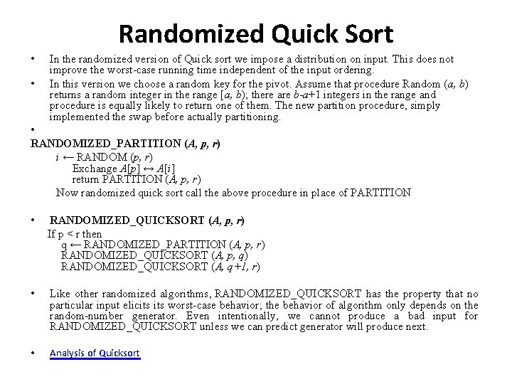
Randomized Quick Sort • In the randomized version of Quick sort we impose a distribution on input. This does not improve the worst-case running time independent of the input ordering. • In this version we choose a random key for the pivot. Assume that procedure Random (a, b) returns a random integer in the range [a, b); there are b-a+1 integers in the range and procedure is equally likely to return one of them. The new partition procedure, simply implemented the swap before actually partitioning. • RANDOMIZED_PARTITION (A, p, r) i ← RANDOM (p, r) Exchange A[p] ↔ A[i] return PARTITION (A, p, r) Now randomized quick sort call the above procedure in place of PARTITION • RANDOMIZED_QUICKSORT (A, p, r) If p < r then q ← RANDOMIZED_PARTITION (A, p, r) RANDOMIZED_QUICKSORT (A, p, q) RANDOMIZED_QUICKSORT (A, q+1, r) • Like other randomized algorithms, RANDOMIZED_QUICKSORT has the property that no particular input elicits worst-case behavior; the behavior of algorithm only depends on the random-number generator. Even intentionally, we cannot produce a bad input for RANDOMIZED_QUICKSORT unless we can predict generator will produce next. • Analysis of Quicksort