Algorithm Design and Recursion Search and Sort Algorithms

Algorithm Design and Recursion Search and Sort Algorithms

Objectives • To understand the basic techniques for analyzing the efficiency of algorithms. • To know what searching is and understand the algorithms for linear and binary search. • To understand the basic principles of recursive definitions and functions and be able to write simple recursive functions.

Objectives • To understand sorting in depth and know the algorithms for selection sort and merge sort. • To appreciate how the analysis of algorithms can demonstrate that some problems are intractable and others are unsolvable.

Searching • Searching is the process of looking for a particular value in a collection. • For example, a program that maintains a membership list for a club might need to look up information for a particular member – this involves some sort of search process.

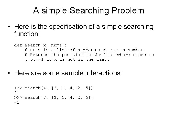
A simple Searching Problem • Here is the specification of a simple searching function: def search(x, nums): # nums is a list of numbers and x is a number # Returns the position in the list where x occurs # or -1 if x is not in the list. • Here are some sample interactions: >>> search(4, [3, 1, 4, 2, 5]) 2 >>> search(7, [3, 1, 4, 2, 5]) -1

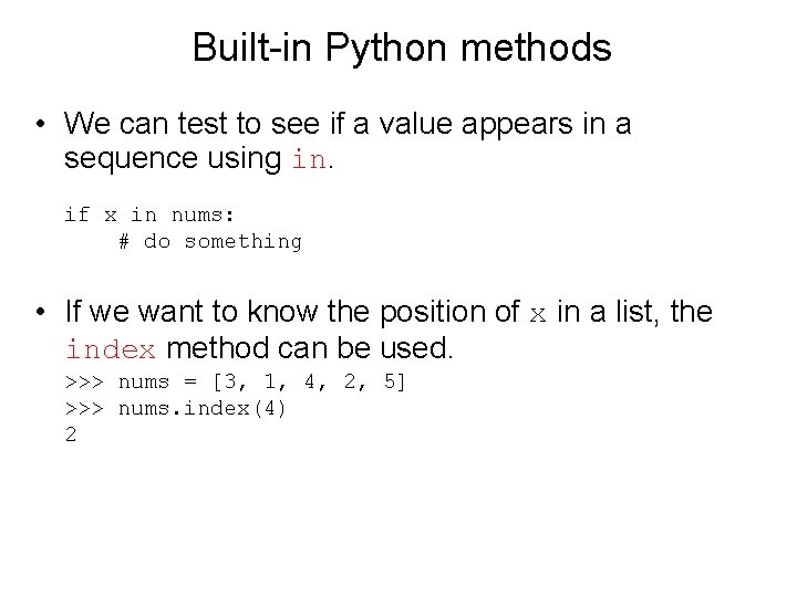
Built-in Python methods • We can test to see if a value appears in a sequence using in. if x in nums: # do something • If we want to know the position of x in a list, the index method can be used. >>> nums = [3, 1, 4, 2, 5] >>> nums. index(4) 2

A Simple Searching Problem • The only difference between our search function and index is that index raises an exception if the target value does not appear in the list. • We could implement search using index by simply catching the exception and returning -1 for that case.

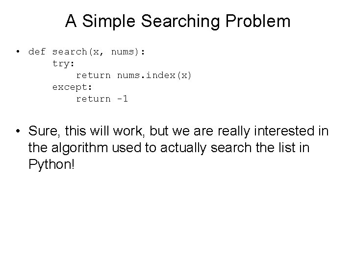
A Simple Searching Problem • def search(x, nums): try: return nums. index(x) except: return -1 • Sure, this will work, but we are really interested in the algorithm used to actually search the list in Python!

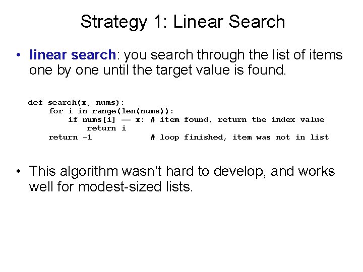
Strategy 1: Linear Search • linear search: you search through the list of items one by one until the target value is found. def search(x, nums): for i in range(len(nums)): if nums[i] == x: # item found, return the index value return i return -1 # loop finished, item was not in list • This algorithm wasn’t hard to develop, and works well for modest-sized lists.

Strategy 1: Linear Search • The Python in and index operations both implement linear searching algorithms. • If the collection of data is very large, it makes sense to organize the data somehow so that each data value doesn’t need to be examined.

Strategy 1: Linear Search • If the data is sorted in ascending order (lowest to highest), we can skip checking some of the data. • As soon as a value is encountered that is greater than the target value, the linear search can be stopped without looking at the rest of the data. • On average, this will save us about half the work.

Strategy 2: Binary Search • If the data is sorted, there is an even better searching strategy – one you probably already know! • Have you ever played the number guessing game, where I pick a number between 1 and 100 and you try to guess it? Each time you guess, I’ll tell you whether your guess is correct, too high, or too low. What strategy do you use?

Strategy 2: Binary Search • Young children might simply guess numbers at random. • Older children may be more systematic, using a linear search of 1, 2, 3, 4, … until the value is found. • Most adults will first guess 50. If told the value is higher, it is in the range 51 -100. The next logical guess is 75.

Strategy 2: Binary Search • Each time we guess the middle of the remaining numbers to try to narrow down the range. • This strategy is called binary search. • Binary means two, and at each step we are diving the remaining group of numbers into two parts.

Strategy 2: Binary Search • We can use the same approach in our binary search algorithm! We can use two variables to keep track of the endpoints of the range in the sorted list where the number could be. • Since the target could be anywhere in the list, initially low is set to the first location in the list, and high is set to the last.

Strategy 2: Binary Search • The heart of the algorithm is a loop that looks at the middle element of the range, comparing it to the value x. • If x is smaller than the middle item, high is moved so that the search is confined to the lower half. • If x is larger than the middle item, low is moved to narrow the search to the upper half.

Strategy 2: Binary Search • The loop terminates when either – x is found – There are no more places to look (low > high)

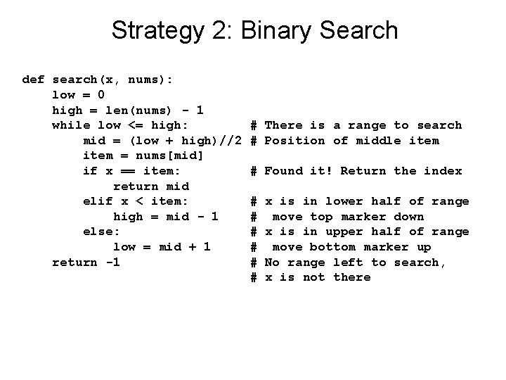
Strategy 2: Binary Search def search(x, nums): low = 0 high = len(nums) - 1 while low <= high: mid = (low + high)//2 item = nums[mid] if x == item: return mid elif x < item: high = mid - 1 else: low = mid + 1 return -1 # There is a range to search # Position of middle item # Found it! Return the index # # # x is in lower half of range move top marker down x is in upper half of range move bottom marker up No range left to search, x is not there

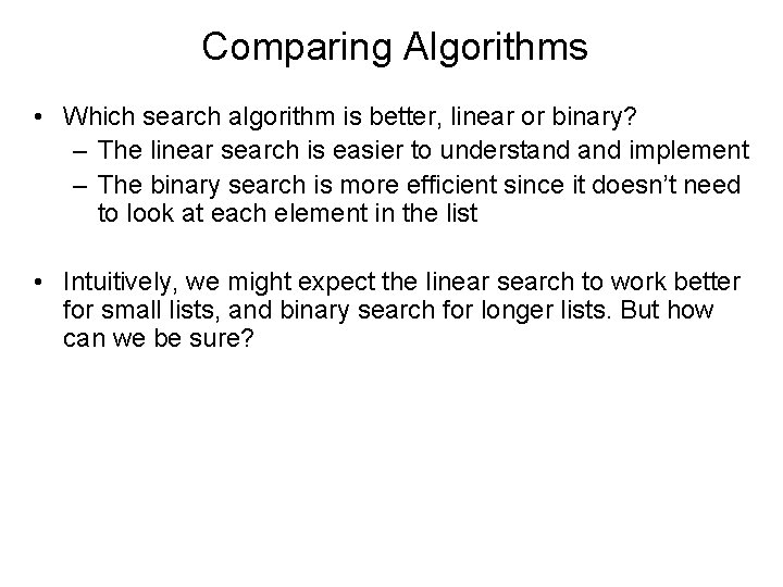
Comparing Algorithms • Which search algorithm is better, linear or binary? – The linear search is easier to understand implement – The binary search is more efficient since it doesn’t need to look at each element in the list • Intuitively, we might expect the linear search to work better for small lists, and binary search for longer lists. But how can we be sure?

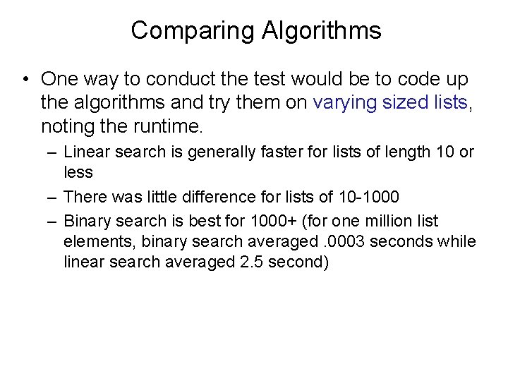
Comparing Algorithms • One way to conduct the test would be to code up the algorithms and try them on varying sized lists, noting the runtime. – Linear search is generally faster for lists of length 10 or less – There was little difference for lists of 10 -1000 – Binary search is best for 1000+ (for one million list elements, binary search averaged. 0003 seconds while linear search averaged 2. 5 second)

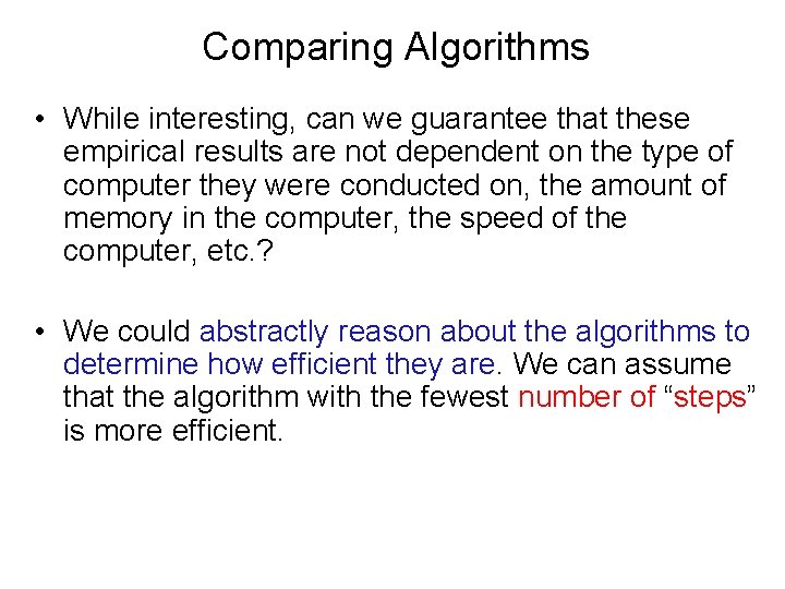
Comparing Algorithms • While interesting, can we guarantee that these empirical results are not dependent on the type of computer they were conducted on, the amount of memory in the computer, the speed of the computer, etc. ? • We could abstractly reason about the algorithms to determine how efficient they are. We can assume that the algorithm with the fewest number of “steps” is more efficient.

Comparing Algorithms • How do we count the number of “steps”? • Computer scientists attack these problems by analyzing the number of steps that an algorithm will take relative to the size or difficulty of the specific problem instance being solved.

Comparing Algorithms • For searching, the difficulty is determined by the size of the collection – it takes more steps to find a number in a collection of a million numbers than it does in a collection of 10 numbers. • How many steps are needed to find a value in a list of size n? • In particular, what happens as n gets very large?

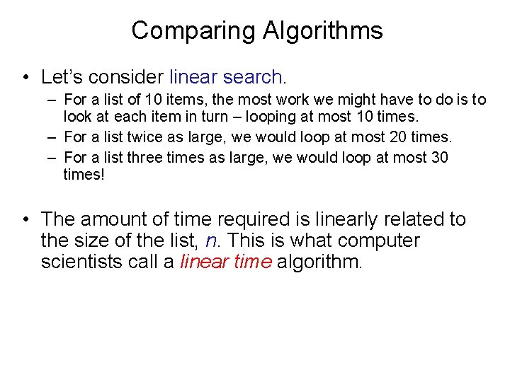
Comparing Algorithms • Let’s consider linear search. – For a list of 10 items, the most work we might have to do is to look at each item in turn – looping at most 10 times. – For a list twice as large, we would loop at most 20 times. – For a list three times as large, we would loop at most 30 times! • The amount of time required is linearly related to the size of the list, n. This is what computer scientists call a linear time algorithm.

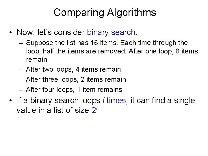
Comparing Algorithms • Now, let’s consider binary search. – Suppose the list has 16 items. Each time through the loop, half the items are removed. After one loop, 8 items remain. – After two loops, 4 items remain. – After three loops, 2 items remain – After four loops, 1 item remains. • If a binary search loops i times, it can find a single value in a list of size 2 i.

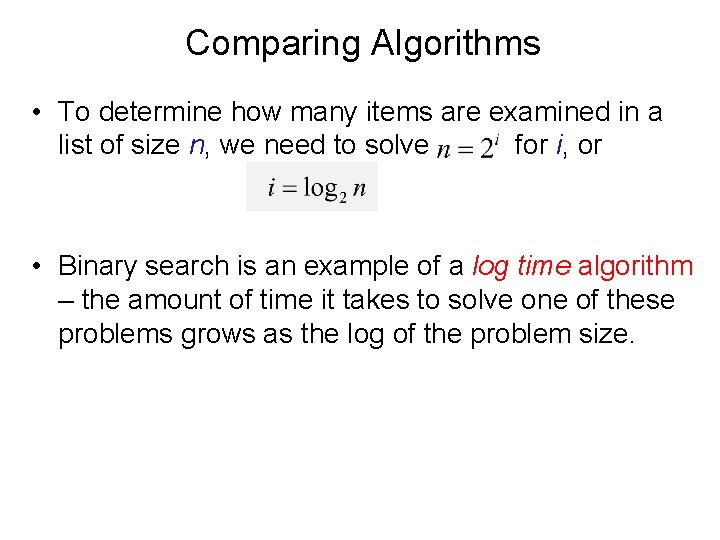
Comparing Algorithms • To determine how many items are examined in a list of size n, we need to solve for i, or • Binary search is an example of a log time algorithm – the amount of time it takes to solve one of these problems grows as the log of the problem size.

Comparing Algorithms • This logarithmic property can be very powerful! • Suppose you have the New York City phone book with 12 million names. You could walk up to a New Yorker and, assuming they are listed in the phone book, make them this proposition: “I’m going to try guessing your name. Each time I guess a name, you tell me if your name comes alphabetically before or after the name I guess. ” How many guesses will you need?

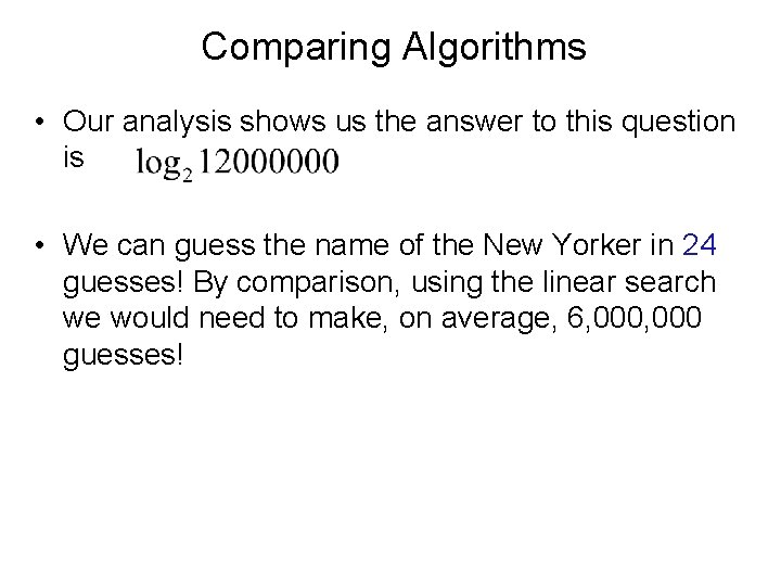
Comparing Algorithms • Our analysis shows us the answer to this question is. • We can guess the name of the New Yorker in 24 guesses! By comparison, using the linear search we would need to make, on average, 6, 000 guesses!

Comparing Algorithms • Earlier, we mentioned that Python uses linear search in its built-in searching methods. Why doesn’t it use binary search? – Binary search requires the data to be sorted – If the data is unsorted, it must be sorted first!

Recursive Problem-Solving • The basic idea between the binary search algorithm was to successfully divide the problem in half. • This technique is known as a divide and conquer approach. • Divide and conquer divides the original problem into subproblems that are smaller versions of the original problem.

Recursive Problem-Solving • In the binary search, the initial range is the entire list. We look at the middle element… if it is the target, we’re done. Otherwise, we continue by performing a binary search on either the top half or bottom half of the list.

Recursive Problem-Solving Algorithm: binary. Search – search for x in nums[low]…nums[high] mid = (low + high)//2 if low > high x is not in nums elsif x < nums[mid] perform binary search for x in nums[low]…nums[mid-1] else perform binary search for x in nums[mid+1]…nums[high] • This version has no loop, and seems to refer to itself! What’s going on? ?

Recursive Definitions • A description of something that refers to itself is called a recursive definition. • In the last example, the binary search algorithm uses its own description – a “call” to binary search “recurs” inside of the definition – hence the label “recursive definition. ”

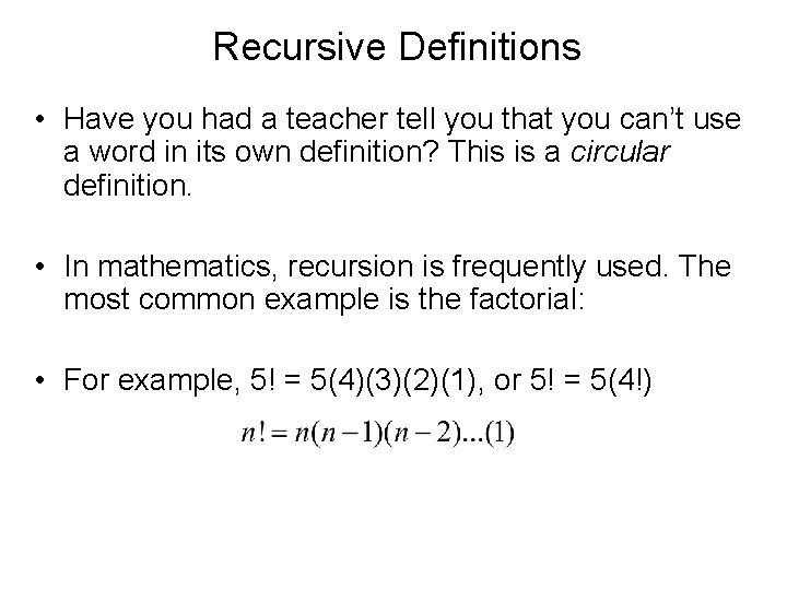
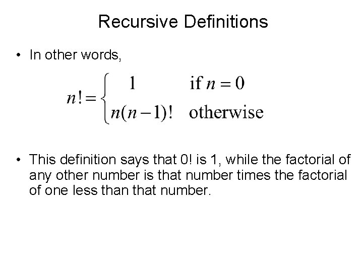
Recursive Definitions • Have you had a teacher tell you that you can’t use a word in its own definition? This is a circular definition. • In mathematics, recursion is frequently used. The most common example is the factorial: • For example, 5! = 5(4)(3)(2)(1), or 5! = 5(4!)

Recursive Definitions • In other words, • This definition says that 0! is 1, while the factorial of any other number is that number times the factorial of one less than that number.

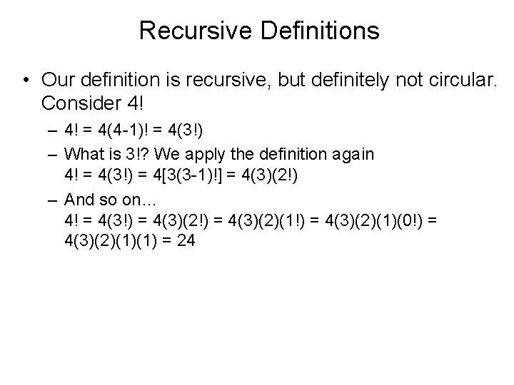
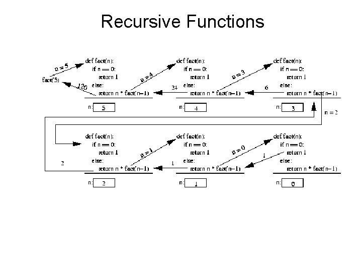
Recursive Definitions • Our definition is recursive, but definitely not circular. Consider 4! – 4! = 4(4 -1)! = 4(3!) – What is 3!? We apply the definition again 4! = 4(3!) = 4[3(3 -1)!] = 4(3)(2!) – And so on… 4! = 4(3!) = 4(3)(2)(1!) = 4(3)(2)(1)(0!) = 4(3)(2)(1)(1) = 24

Recursive Definitions • Factorial is not circular because we eventually get to 0!, whose definition does not rely on the definition of factorial and is just 1. This is called a base case for the recursion. • When the base case is encountered, we get a closed expression that can be directly computed.

Recursive Definitions • All good recursive definitions have these two key characteristics: – There are one or more base cases for which no recursion is applied. – All chains of recursion eventually end up at one of the base cases. • The simplest way for these two conditions to occur is for each recursion to act on a smaller version of the original problem. A very small version of the original problem that can be solved without recursion becomes the base case.

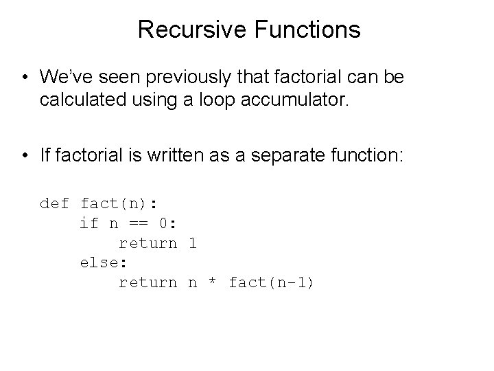
Recursive Functions • We’ve seen previously that factorial can be calculated using a loop accumulator. • If factorial is written as a separate function: def fact(n): if n == 0: return 1 else: return n * fact(n-1)

Recursive Functions

Example: String Reversal • Python lists have a built-in method that can be used to reverse the list. What if you wanted to reverse a string? • If you wanted to program this yourself, one way to do it would be to convert the string into a list of characters, reverse the list, and then convert it back into a string.

Example: String Reversal • Using recursion, we can calculate the reverse of a string without the intermediate list step. • Think of a string as a recursive object: – Divide it up into a first character and “all the rest” – Reverse the “rest” and append the first character to the end of it

Example: String Reversal • def reverse(s): return reverse(s[1: ]) + s[0] • The slice s[1: ] returns all but the first character of the string. • We reverse this slice and then concatenate the first character (s[0]) onto the end.

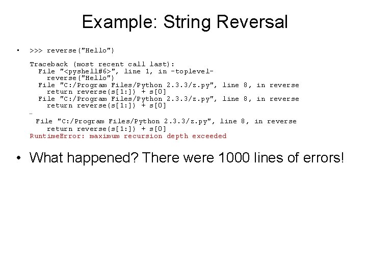
Example: String Reversal • >>> reverse("Hello") Traceback (most recent call last): File "<pyshell#6>", line 1, in -toplevelreverse("Hello") File "C: /Program Files/Python 2. 3. 3/z. py", line 8, in reverse return reverse(s[1: ]) + s[0] … File "C: /Program Files/Python 2. 3. 3/z. py", line 8, in reverse return reverse(s[1: ]) + s[0] Runtime. Error: maximum recursion depth exceeded • What happened? There were 1000 lines of errors!

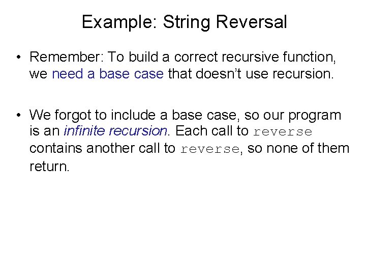
Example: String Reversal • Remember: To build a correct recursive function, we need a base case that doesn’t use recursion. • We forgot to include a base case, so our program is an infinite recursion. Each call to reverse contains another call to reverse, so none of them return.

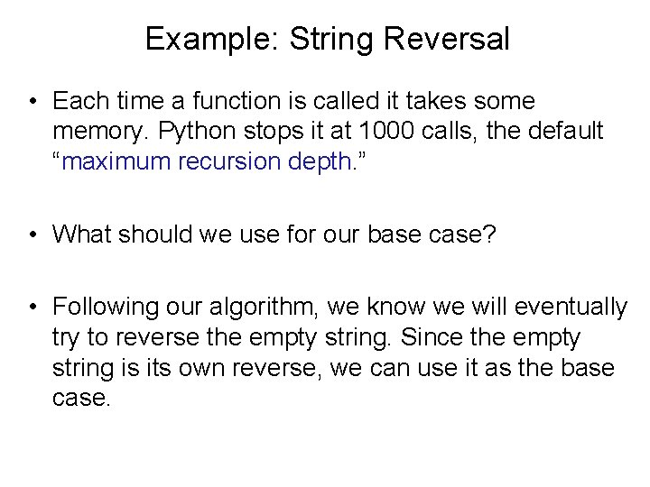
Example: String Reversal • Each time a function is called it takes some memory. Python stops it at 1000 calls, the default “maximum recursion depth. ” • What should we use for our base case? • Following our algorithm, we know we will eventually try to reverse the empty string. Since the empty string is its own reverse, we can use it as the base case.

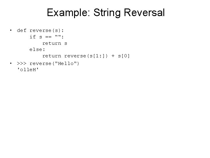
Example: String Reversal • def reverse(s): if s == "": return s else: return reverse(s[1: ]) + s[0] • >>> reverse("Hello") 'olle. H'

Example: Anagrams • An anagram is formed by rearranging the letters of a word. • Anagram formation is a special case of generating all permutations (rearrangements) of a sequence, a problem that is seen frequently in mathematics and computer science.

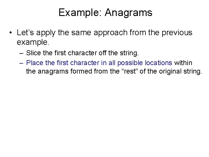
Example: Anagrams • Let’s apply the same approach from the previous example. – Slice the first character off the string. – Place the first character in all possible locations within the anagrams formed from the “rest” of the original string.

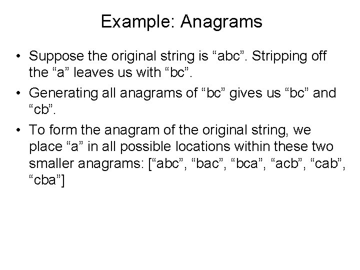
Example: Anagrams • Suppose the original string is “abc”. Stripping off the “a” leaves us with “bc”. • Generating all anagrams of “bc” gives us “bc” and “cb”. • To form the anagram of the original string, we place “a” in all possible locations within these two smaller anagrams: [“abc”, “bac”, “bca”, “acb”, “cab”, “cba”]

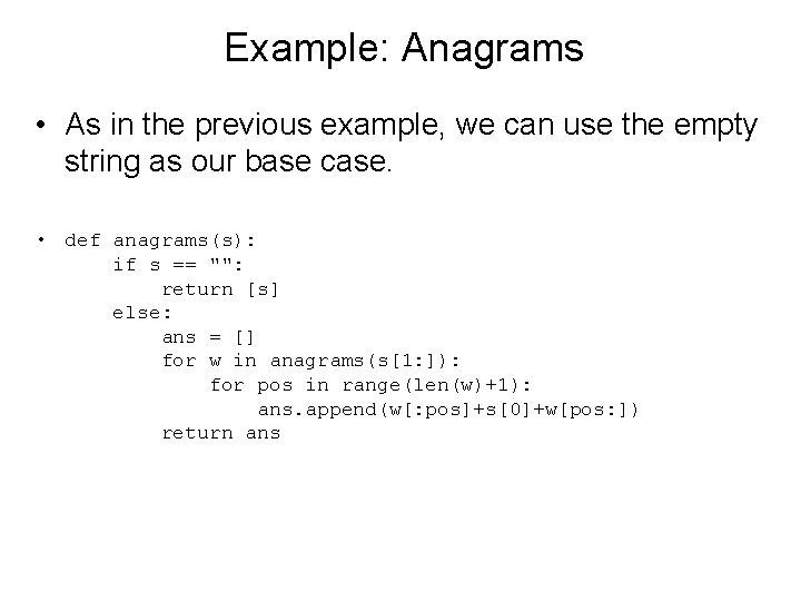
Example: Anagrams • As in the previous example, we can use the empty string as our base case. • def anagrams(s): if s == "": return [s] else: ans = [] for w in anagrams(s[1: ]): for pos in range(len(w)+1): ans. append(w[: pos]+s[0]+w[pos: ]) return ans

Example: Anagrams • w[: pos]+s[0]+w[pos: ] – w[: pos] gives the part of w up to, but not including, pos. – w[pos: ] gives everything from pos to the end. – Inserting s[0] between them effectively inserts it into w at pos.

Example: Anagrams • A list is used to accumulate results. • The outer for loop iterates through each anagram of the tail of s. • The inner loop goes through each position in the anagram and creates a new string with the original first character inserted into that position. • The inner loop goes up to len(w)+1 so the new character can be added at the end of the anagram.

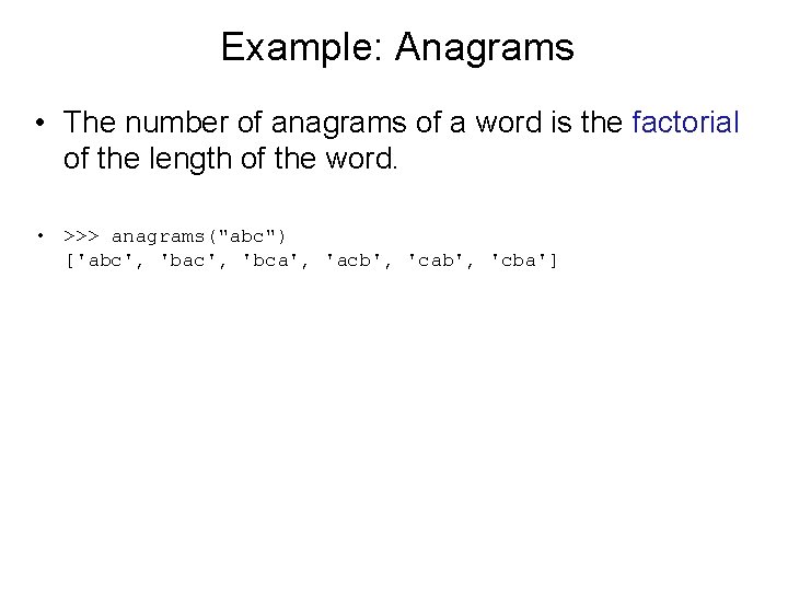
Example: Anagrams • The number of anagrams of a word is the factorial of the length of the word. • >>> anagrams("abc") ['abc', 'bac', 'bca', 'acb', 'cab', 'cba']

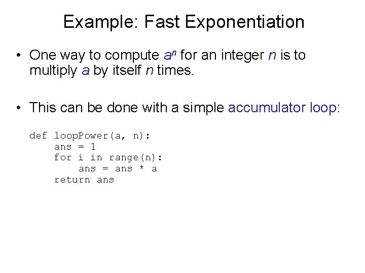
Example: Fast Exponentiation • One way to compute an for an integer n is to multiply a by itself n times. • This can be done with a simple accumulator loop: def loop. Power(a, n): ans = 1 for i in range(n): ans = ans * a return ans

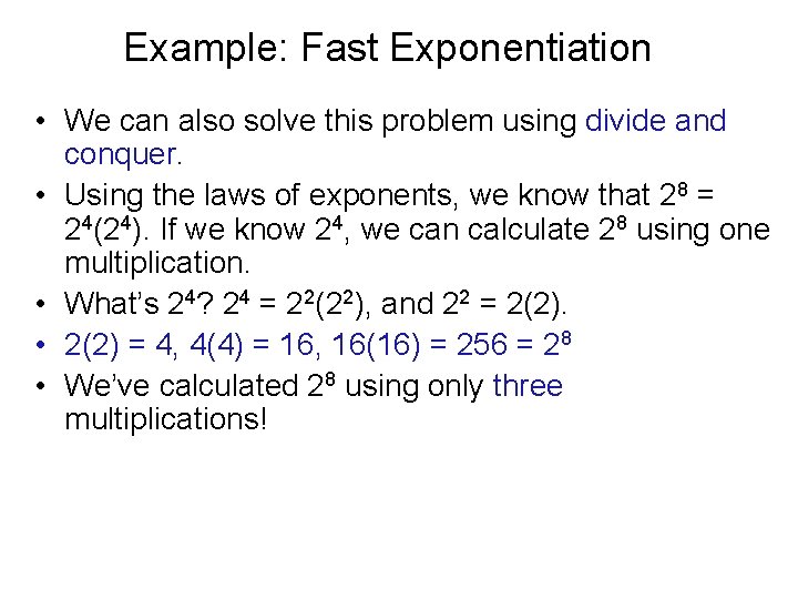
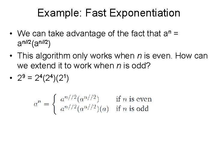
Example: Fast Exponentiation • We can also solve this problem using divide and conquer. • Using the laws of exponents, we know that 28 = 24(24). If we know 24, we can calculate 28 using one multiplication. • What’s 24? 24 = 22(22), and 22 = 2(2). • 2(2) = 4, 4(4) = 16, 16(16) = 256 = 28 • We’ve calculated 28 using only three multiplications!

Example: Fast Exponentiation • We can take advantage of the fact that an = an//2(an//2) • This algorithm only works when n is even. How can we extend it to work when n is odd? • 29 = 24(24)(21)

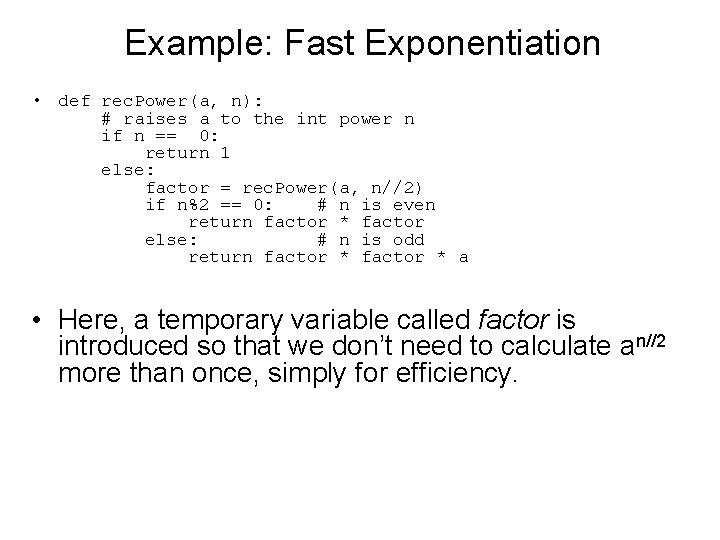
Example: Fast Exponentiation • def rec. Power(a, n): # raises a to the int power n if n == 0: return 1 else: factor = rec. Power(a, n//2) if n%2 == 0: # n is even return factor * factor else: # n is odd return factor * a • Here, a temporary variable called factor is introduced so that we don’t need to calculate an//2 more than once, simply for efficiency.

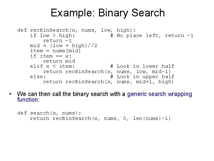
Example: Binary Search • Now that you’ve seen some recursion examples, you’re ready to look at doing binary searches recursively. • Remember: we look at the middle value first, then we either search the lower half or upper half of the array. • The base cases are when we can stop searching, namely, when the target is found or when we’ve run out of places to look.

Example: Binary Search def rec. Bin. Search(x, nums, low, if low > high: # return -1 mid = (low + high)//2 item = nums[mid] if item == x: return mid elif x < item: # return rec. Bin. Search(x, else: # return rec. Bin. Search(x, high): No place left, return -1 Look in lower half nums, low, mid-1) Look in upper half nums, mid+1, high) • We can then call the binary search with a generic search wrapping function: def search(x, nums): return rec. Bin. Search(x, nums, 0, len(nums)-1)

Recursion vs. Iteration • There are similarities between iteration (looping) and recursion. • In fact, anything that can be done with a loop can be done with a simple recursive function! Some programming languages use recursion exclusively. • Some problems that are simple to solve with recursion are quite difficult to solve with loops (e. g. tree traversal)

Recursion vs. Iteration • In the factorial and binary search problems, the looping and recursive solutions use roughly the same algorithms, and their efficiency is nearly the same. • In the exponentiation problem, two different algorithms are used. The looping version takes linear time to complete, while the recursive version executes in log time. The difference between them is like the difference between a linear and binary search.

Recursion vs. Iteration • So… will recursive solutions always be as efficient or more efficient than their iterative counterpart? • The Fibonacci sequence is the sequence of numbers 1, 1, 2, 3, 5, 8, … – The sequence starts with two 1’s – Successive numbers are calculated by finding the sum of the previous two

Recursion vs. Iteration • Loop version: – Let’s use two variables, curr and prev, to calculate the next number in the sequence. – Once this is done, we set prev equal to curr, and set curr equal to the just-calculated number. – All we need to do is to put this into a loop to execute the right number of times!

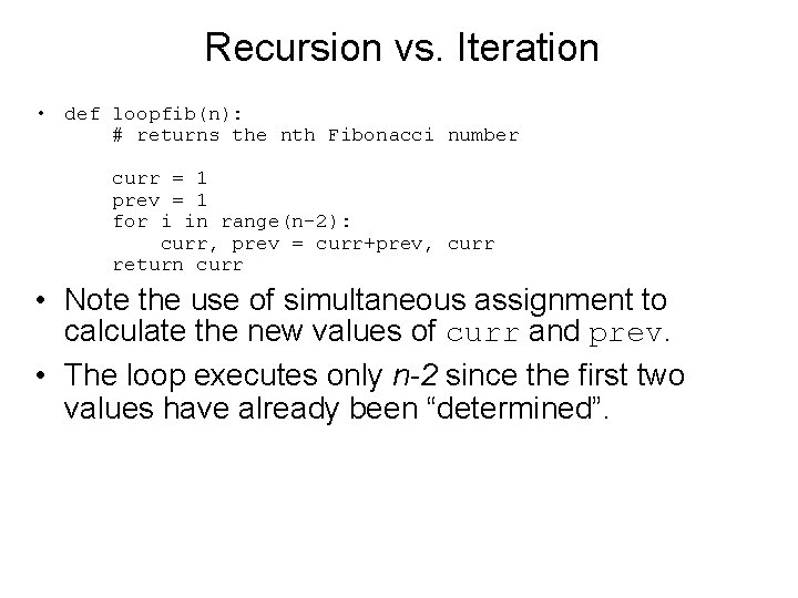
Recursion vs. Iteration • def loopfib(n): # returns the nth Fibonacci number curr = 1 prev = 1 for i in range(n-2): curr, prev = curr+prev, curr return curr • Note the use of simultaneous assignment to calculate the new values of curr and prev. • The loop executes only n-2 since the first two values have already been “determined”.

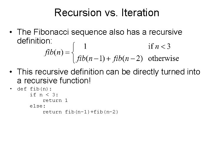
Recursion vs. Iteration • The Fibonacci sequence also has a recursive definition: • This recursive definition can be directly turned into a recursive function! • def fib(n): if n < 3: return 1 else: return fib(n-1)+fib(n-2)

Recursion vs. Iteration • This function obeys the rules that we’ve set out. – The recursion is always based on smaller values. – There is a non-recursive base case. • So, this function will work great, won’t it? – Sort of…

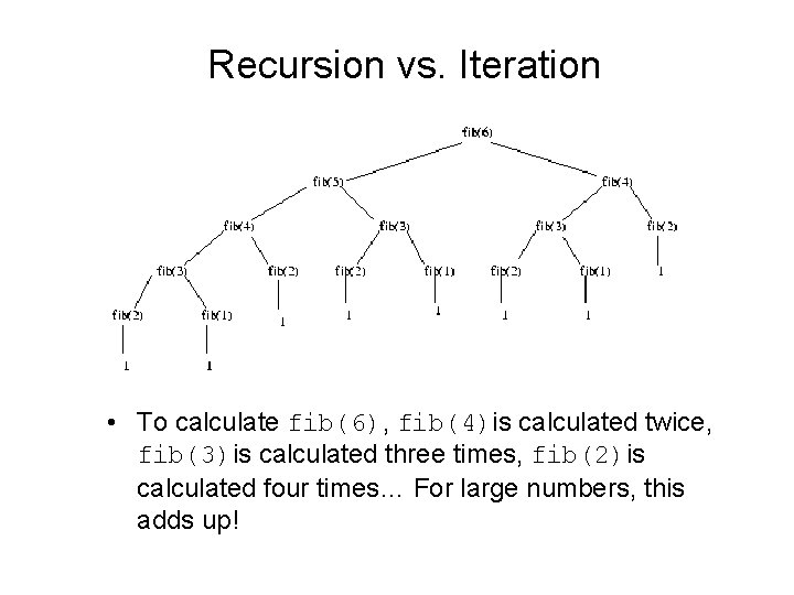
Recursion vs. Iteration • To calculate fib(6), fib(4)is calculated twice, fib(3)is calculated three times, fib(2)is calculated four times… For large numbers, this adds up!

Recursion vs. Iteration • Recursion is another tool in your problem-solving toolbox. • Sometimes recursion provides a good solution because it is more elegant or efficient than a looping version. • At other times, when both algorithms are quite similar, the edge goes to the looping solution on the basis of speed. • Avoid the recursive solution if it is terribly inefficient, unless you can’t come up with an iterative solution (which sometimes happens!)

Sorting Algorithms • The basic sorting problem is to take a list and rearrange it so that the values are in increasing (or nondecreasing) order.

Naive Sorting: Selection Sort • To start out, pretend you’re the computer, and you’re given a shuffled stack of index cards, each with a number. How would you put the cards back in order?

Naive Sorting: Selection Sort • One simple method is to look through the deck to find the smallest value and place that value at the front of the stack. • Then go through, find the next smallest number in the remaining cards, place it behind the smallest card at the front. • Rinse, lather, repeat, until the stack is in sorted order!

Naive Sorting: Selection Sort • The algorithm has a loop, and each time through the loop the smallest remaining element is selected and moved into its proper position. – For n elements, we find the smallest value and put it in the 0 th position. – Then we find the smallest remaining value from position 1 – (n-1) and put it into position 1. – The smallest value from position 2 – (n-1) goes in position 2. – Etc.

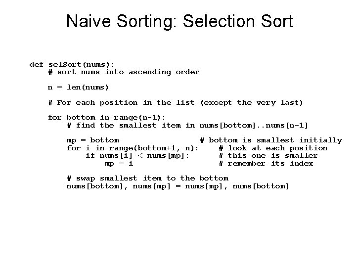
Naive Sorting: Selection Sort def sel. Sort(nums): # sort nums into ascending order n = len(nums) # For each position in the list (except the very last) for bottom in range(n-1): # find the smallest item in nums[bottom]. . nums[n-1] mp = bottom # bottom is smallest initially for i in range(bottom+1, n): # look at each position if nums[i] < nums[mp]: # this one is smaller mp = i # remember its index # swap smallest item to the bottom nums[bottom], nums[mp] = nums[mp], nums[bottom]

Naive Sorting: Selection Sort • The selection sort is easy to write and works well for moderate-sized lists, but is not terribly efficient. We’ll analyze this algorithm in a little bit.

Divide and Conquer: Merge Sort • We’ve seen how divide and conquer works in other types of problems. How could we apply it to sorting? • Say you and your friend have a deck of shuffled cards you’d like to sort. Each of you could take half the cards and sort them. Then all you’d need is a way to recombine the two sorted stacks!

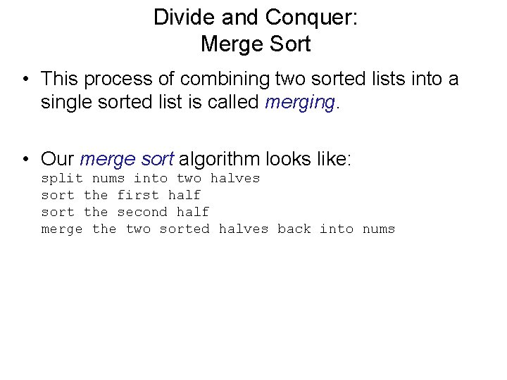
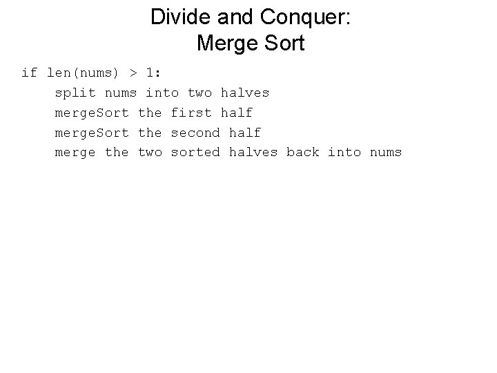
Divide and Conquer: Merge Sort • This process of combining two sorted lists into a single sorted list is called merging. • Our merge sort algorithm looks like: split nums into two halves sort the first half sort the second half merge the two sorted halves back into nums

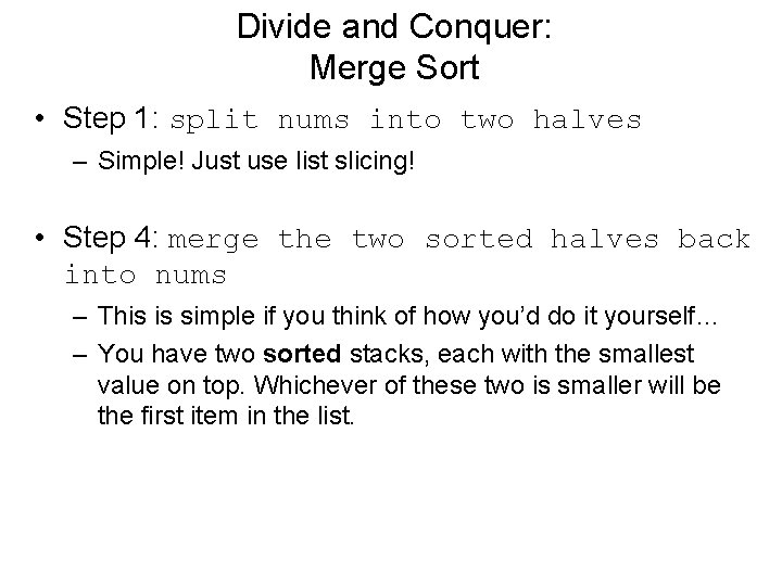
Divide and Conquer: Merge Sort • Step 1: split nums into two halves – Simple! Just use list slicing! • Step 4: merge the two sorted halves back into nums – This is simple if you think of how you’d do it yourself… – You have two sorted stacks, each with the smallest value on top. Whichever of these two is smaller will be the first item in the list.

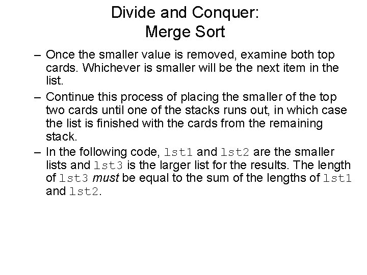
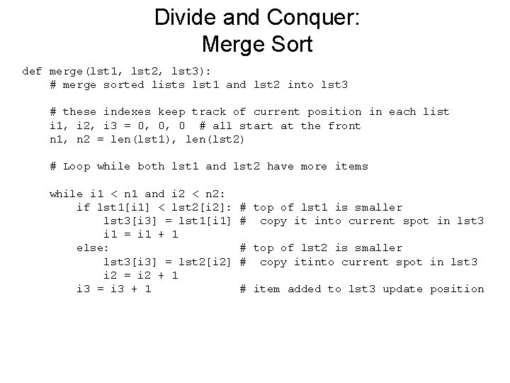
Divide and Conquer: Merge Sort – Once the smaller value is removed, examine both top cards. Whichever is smaller will be the next item in the list. – Continue this process of placing the smaller of the top two cards until one of the stacks runs out, in which case the list is finished with the cards from the remaining stack. – In the following code, lst 1 and lst 2 are the smaller lists and lst 3 is the larger list for the results. The length of lst 3 must be equal to the sum of the lengths of lst 1 and lst 2.

Divide and Conquer: Merge Sort def merge(lst 1, lst 2, lst 3): # merge sorted lists lst 1 and lst 2 into lst 3 # these indexes keep track of current position in each list i 1, i 2, i 3 = 0, 0, 0 # all start at the front n 1, n 2 = len(lst 1), len(lst 2) # Loop while both lst 1 and lst 2 have more items while i 1 < n 1 and i 2 < n 2: if lst 1[i 1] < lst 2[i 2]: lst 3[i 3] = lst 1[i 1] i 1 = i 1 + 1 else: lst 3[i 3] = lst 2[i 2] i 2 = i 2 + 1 i 3 = i 3 + 1 # top of lst 1 is smaller # copy it into current spot in lst 3 # top of lst 2 is smaller # copy itinto current spot in lst 3 # item added to lst 3 update position

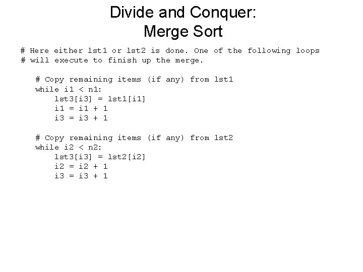
Divide and Conquer: Merge Sort # Here either lst 1 or lst 2 is done. One of the following loops # will execute to finish up the merge. # Copy remaining items (if any) from lst 1 while i 1 < n 1: lst 3[i 3] = lst 1[i 1] i 1 = i 1 + 1 i 3 = i 3 + 1 # Copy remaining items (if any) from lst 2 while i 2 < n 2: lst 3[i 3] = lst 2[i 2] i 2 = i 2 + 1 i 3 = i 3 + 1

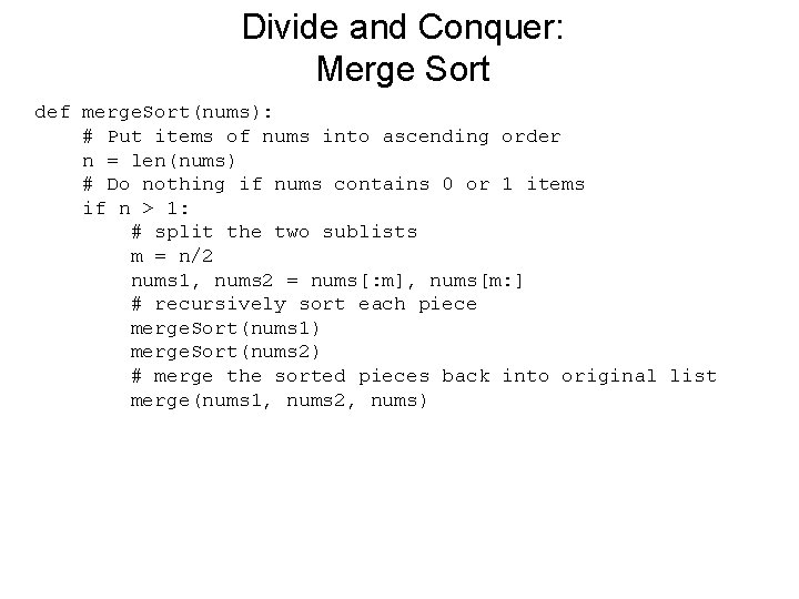
Divide and Conquer: Merge Sort • We can slice a list in two, and we can merge these new sorted lists back into a single list. How are we going to sort the smaller lists? • We are trying to sort a list, and the algorithm requires two smaller sorted lists… this sounds like a job for recursion!

Divide and Conquer: Merge Sort • We need to find at least one base case that does not require a recursive call, and we also need to ensure that recursive calls are always made on smaller versions of the original problem. • For the latter, we know this is true since each time we are working on halves of the previous list.

Divide and Conquer: Merge Sort • Eventually, the lists will be halved into lists with a single element each. What do we know about a list with a single item? • It’s already sorted!! We have our base case! When the length of the list is less than 2, we do nothing.

Divide and Conquer: Merge Sort if len(nums) > 1: split nums into two halves merge. Sort the first half merge. Sort the second half merge the two sorted halves back into nums

Divide and Conquer: Merge Sort def merge. Sort(nums): # Put items of nums into ascending order n = len(nums) # Do nothing if nums contains 0 or 1 items if n > 1: # split the two sublists m = n/2 nums 1, nums 2 = nums[: m], nums[m: ] # recursively sort each piece merge. Sort(nums 1) merge. Sort(nums 2) # merge the sorted pieces back into original list merge(nums 1, nums 2, nums)

Comparing Sorts • We now have two sorting algorithms. Which one should we use? • The difficulty of sorting a list depends on the size of the list. We need to figure out how many steps each of our sorting algorithms requires as a function of the size of the list to be sorted.

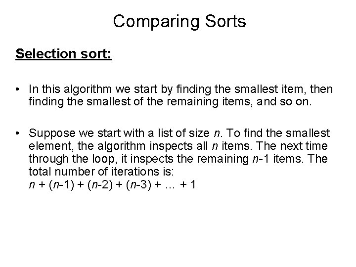
Comparing Sorts Selection sort: • In this algorithm we start by finding the smallest item, then finding the smallest of the remaining items, and so on. • Suppose we start with a list of size n. To find the smallest element, the algorithm inspects all n items. The next time through the loop, it inspects the remaining n-1 items. The total number of iterations is: n + (n-1) + (n-2) + (n-3) + … + 1

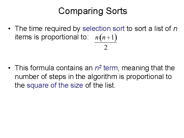
Comparing Sorts • The time required by selection sort to sort a list of n items is proportional to: • This formula contains an n 2 term, meaning that the number of steps in the algorithm is proportional to the square of the size of the list.

Comparing Sorts • If the size of a list doubles, it will take four times as long to sort. Tripling the size will take nine times longer to sort! • Computer scientists call this a quadratic or n 2 algorithm.

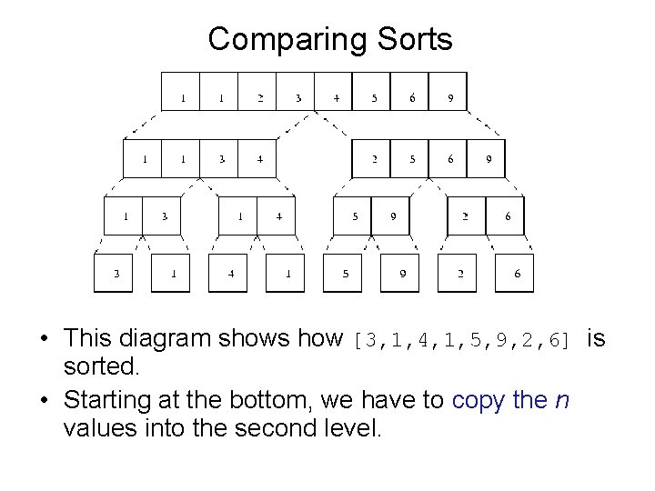
Comparing Sorts • In the case of the merge sort, a list is divided into two pieces and each piece is sorted before merging them back together. The real place where the sorting occurs is in the merge function.

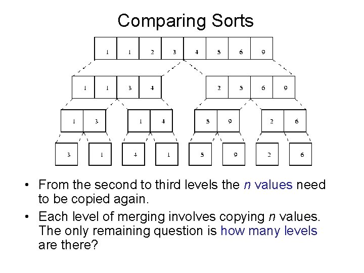
Comparing Sorts • This diagram shows how [3, 1, 4, 1, 5, 9, 2, 6] is sorted. • Starting at the bottom, we have to copy the n values into the second level.

Comparing Sorts • From the second to third levels the n values need to be copied again. • Each level of merging involves copying n values. The only remaining question is how many levels are there?

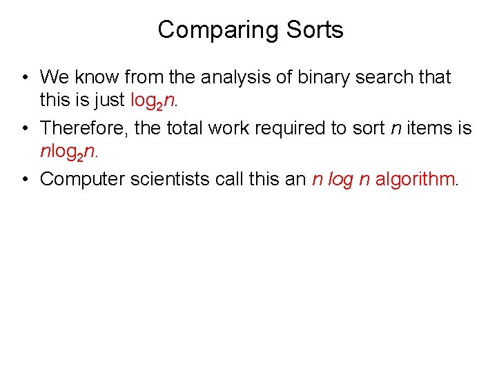
Comparing Sorts • We know from the analysis of binary search that this is just log 2 n. • Therefore, the total work required to sort n items is nlog 2 n. • Computer scientists call this an n log n algorithm.

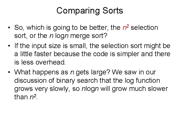
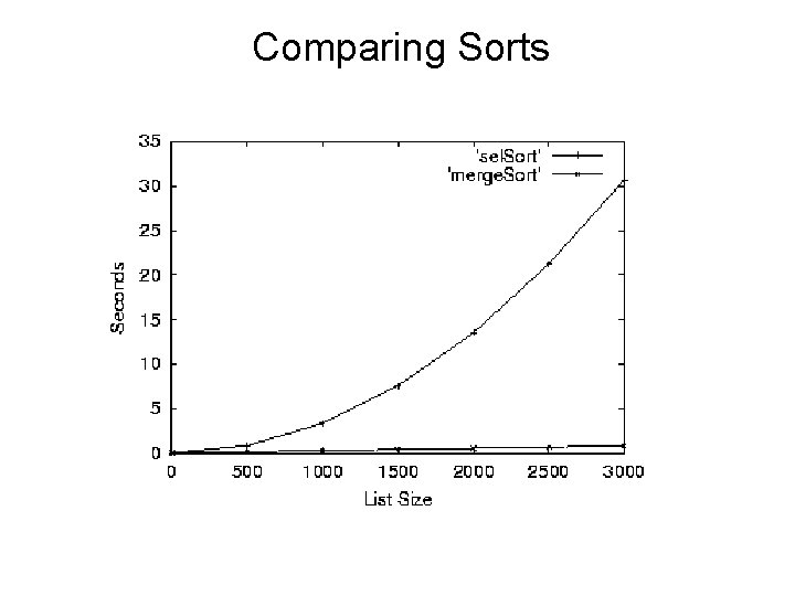
Comparing Sorts • So, which is going to be better, the n 2 selection sort, or the n logn merge sort? • If the input size is small, the selection sort might be a little faster because the code is simpler and there is less overhead. • What happens as n gets large? We saw in our discussion of binary search that the log function grows very slowly, so nlogn will grow much slower than n 2.

Comparing Sorts

Hard Problems • Using divide-and-conquer we could design efficient algorithms for searching and sorting problems. • Divide and conquer and recursion are very powerful techniques for algorithm design. • Not all problems have efficient solutions!

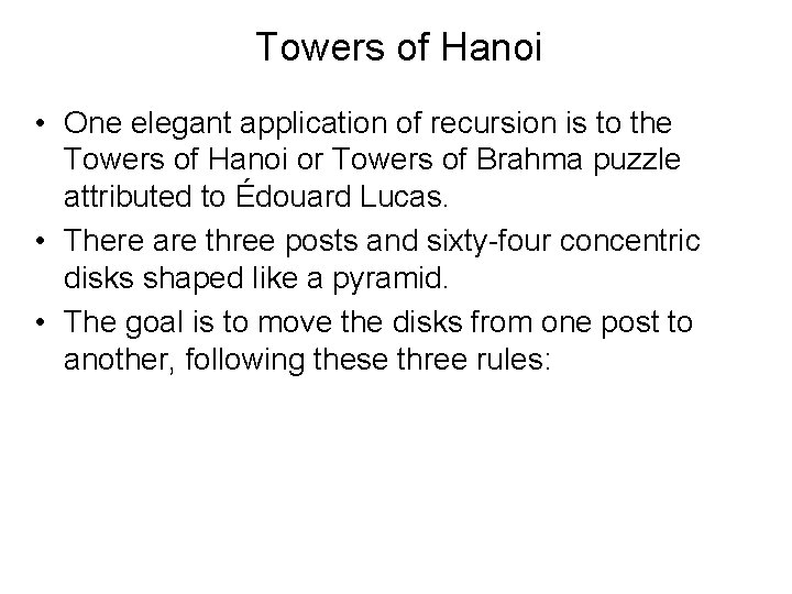
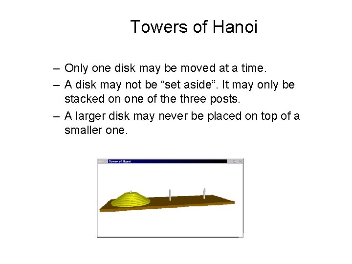
Towers of Hanoi • One elegant application of recursion is to the Towers of Hanoi or Towers of Brahma puzzle attributed to Édouard Lucas. • There are three posts and sixty-four concentric disks shaped like a pyramid. • The goal is to move the disks from one post to another, following these three rules:

Towers of Hanoi – Only one disk may be moved at a time. – A disk may not be “set aside”. It may only be stacked on one of the three posts. – A larger disk may never be placed on top of a smaller one.

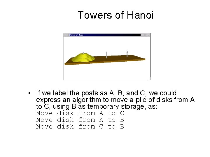
Towers of Hanoi • If we label the posts as A, B, and C, we could express an algorithm to move a pile of disks from A to C, using B as temporary storage, as: Move disk from A to C Move disk from A to B Move disk from C to B

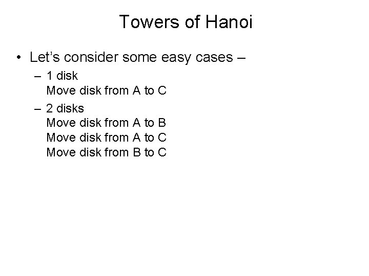
Towers of Hanoi • Let’s consider some easy cases – – 1 disk Move disk from A to C – 2 disks Move disk from A to B Move disk from A to C Move disk from B to C

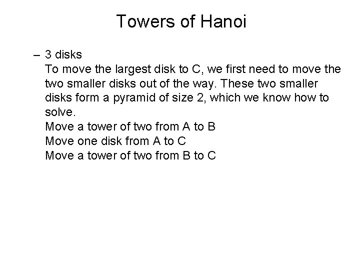
Towers of Hanoi – 3 disks To move the largest disk to C, we first need to move the two smaller disks out of the way. These two smaller disks form a pyramid of size 2, which we know how to solve. Move a tower of two from A to B Move one disk from A to C Move a tower of two from B to C

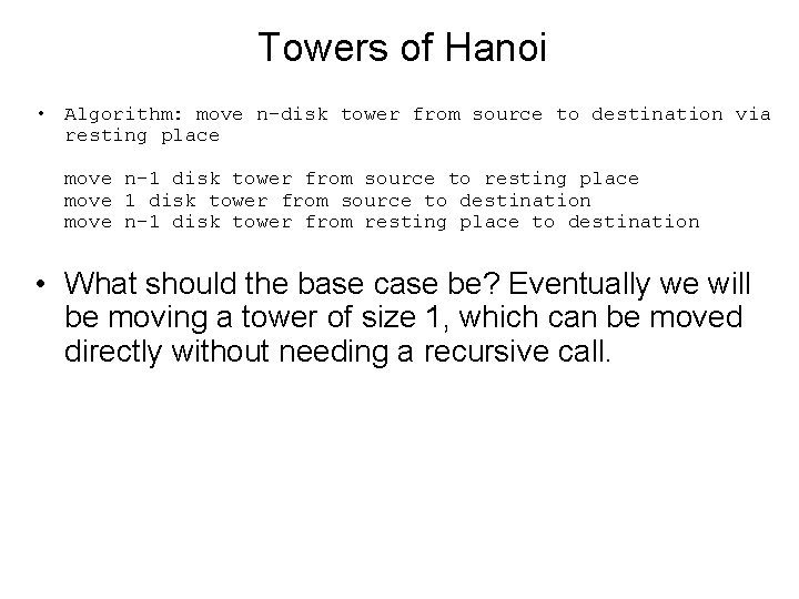
Towers of Hanoi • Algorithm: move n-disk tower from source to destination via resting place move n-1 disk tower from source to resting place move 1 disk tower from source to destination move n-1 disk tower from resting place to destination • What should the base case be? Eventually we will be moving a tower of size 1, which can be moved directly without needing a recursive call.

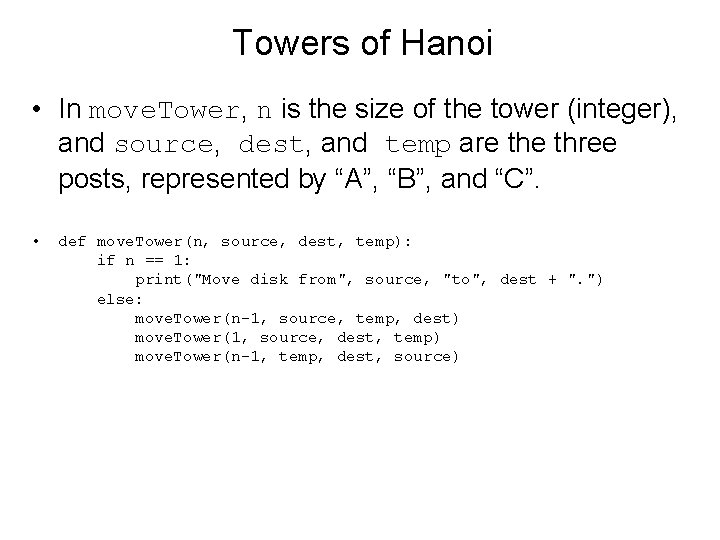
Towers of Hanoi • In move. Tower, n is the size of the tower (integer), and source, dest, and temp are three posts, represented by “A”, “B”, and “C”. • def move. Tower(n, source, dest, temp): if n == 1: print("Move disk from", source, "to", dest + ". ") else: move. Tower(n-1, source, temp, dest) move. Tower(1, source, dest, temp) move. Tower(n-1, temp, dest, source)

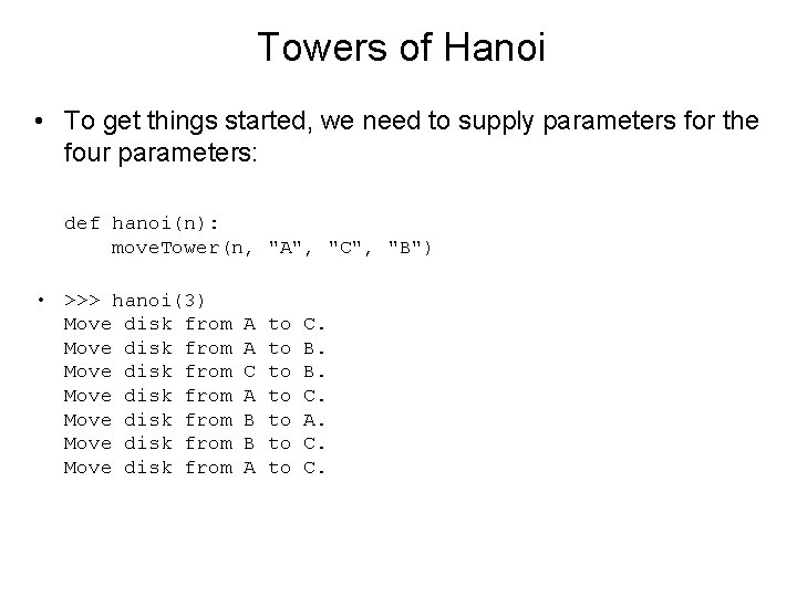
Towers of Hanoi • To get things started, we need to supply parameters for the four parameters: def hanoi(n): move. Tower(n, "A", "C", "B") • >>> hanoi(3) Move disk from Move disk from A A C A B B A to to C. B. B. C. A. C. C.

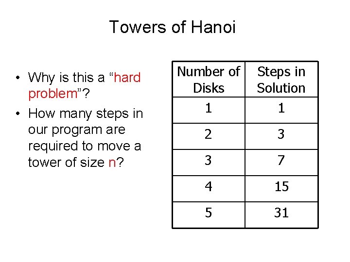
Towers of Hanoi • Why is this a “hard problem”? • How many steps in our program are required to move a tower of size n? Number of Disks 1 Steps in Solution 1 2 3 3 7 4 15 5 31

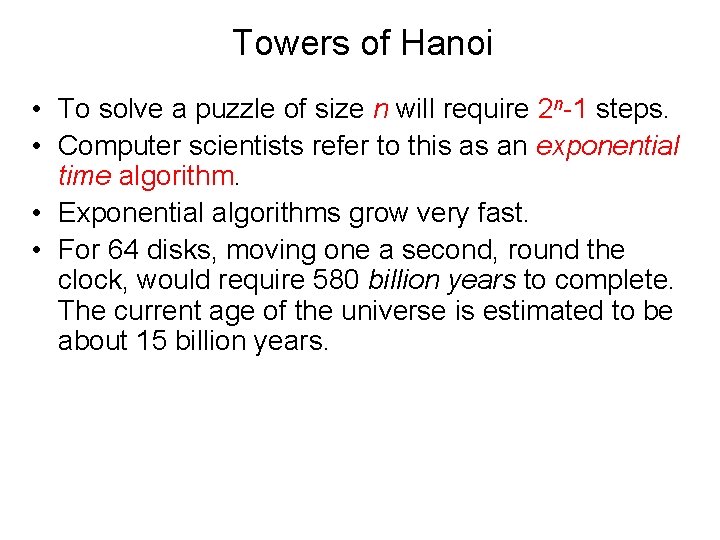
Towers of Hanoi • To solve a puzzle of size n will require 2 n-1 steps. • Computer scientists refer to this as an exponential time algorithm. • Exponential algorithms grow very fast. • For 64 disks, moving one a second, round the clock, would require 580 billion years to complete. The current age of the universe is estimated to be about 15 billion years.

Towers of Hanoi • Even though the algorithm for Towers of Hanoi is easy to express, it belongs to a class of problems known as intractable problems – those that require too many computing resources (either time or memory) to be solved except for the simplest of cases.

Conclusions • Computer Science is more than programming! • Think about algorithms and implementations.

Acknowledgement • Slides are due to. John Zelle