Algorithm Analysis Objectives l Determine the running time

Algorithm Analysis

Objectives l Determine the running time of simple algorithms in the: ¡ ¡ ¡ Best case Average case Worst case Profile algorithms l Understand the mathematical basis of O notation l Use O notation to measure the running time of algorithms l

Algorithm Analysis It is important to be able to describe the efficiency of algorithms l Choosing an appropriate algorithm can make an enormous difference in the usability of a system e. g. l ¡ ¡ ¡ Government and corporate databases with many millions of records, which are accessed frequently Online search engines Real time systems (from air traffic control systems to computer games) where near instantaneous response is required

Best, Average and Worst Case l The amount of work performed by an algorithm may vary based on its input ¡ l This is frequently the case (but not always) Algorithm efficiency is often calculated for three, general, cases of input ¡ ¡ ¡ Best case Average (or “usual”) case Worst case

Measuring Algorithms l It is possible to count the number of operations that an algorithm performs ¡ ¡ l Either by a careful visual walkthrough of the algorithm or by Printing the number of times that each line executes (profiling) It is also possible to time algorithms ¡ ¡ System. current. Time. Millis() returns the current time so can easily be used to measure the running time of an algorithm More sophisticated timer classes exist

Timing Algorithms l It can be very useful to time how long an algorithm takes to run ¡ l In some cases it may be essential to know how long a particular algorithm takes on a particular system However, it is not a good general method for comparing algorithms ¡ Running time is affected by numerous factors l l CPU speed, memory, specialized hardware (e. g. graphics card) Operating system, system configuration (e. g. virtual memory), algorithm implementation (including language) Other tasks (i. e. what other programs are running), timing of system tasks (e. g. memory management) …

Barometer Instructions l For general comparative purposes we will count (rather than time) the number of operations that an algorithm performs ¡ l Note that this does not mean that actual running time should be ignored! Count the number of times that an algorithm executes its barometer instruction ¡ ¡ The instruction that is executed the most number of time in an algorithm The results are usually proportional to running time

Example: Linear Search Iterate through an array of n items searching for the target item l The barometer instruction is equality checking (or “comparisons” for short) l ¡ ¡ l x. equals(arr[i]); //for an object or x == arr[i]; //for a primitive type How many comparisons does linear search do?

Linear Search Comparisons Best case: 1 comparison (where the target is found at the start of the array) l Worst case: n comparisons where: l l ¡ The target is not in the array or ¡ The target is at the last position in the array Average case: ¡ ¡ Seems like it should be roughly n/2 But the analysis can get quite tricky

Linear Search: Average Case l Before calculating the number of comparisons made in the average case we need more information ¡ ¡ l How often is the target actually going to be in the array? If x is in the array, what is the chance that it is at a particular location? We can make assumptions about these two things but it is important to realize that these assumptions may not hold for a particular use of linear search ¡ ¡ Assume that the target is in the array 50% of the time and that Assume that if the target is in the array it has an equal chance of being at any location (so there is a probability of 1/n that the target is at some location i)

Linear Search: Average Case l Work done if x is not in the array: ¡ n comparisons l l happens with probability of 0. 5 from the first assumption Work done if x is in the array: ¡ 1 comparison if x is at the 1 st location l ¡ ¡ ¡ happens with probability 0. 5 * 1/n from the first and second assumptions 2 comparisons if x is at the 2 nd location i comparisons if x is at the ith location Take the weighted average of these values to determine the total expected number of comparisons l l E = 1*1/n + 2*1/n + 3*1/n + … + n * 1/n or E = (n + 1) / 2

Linear Search: Average Case l 50% of the time n comparisons are made, when x is not in the array l 50% of the time, (n + 1)/2 comparisons are made, when x is in the array l The weighted average of these two amounts gives: ¡ ¡ ¡ l 0. 5 * n + (0. 5 * (n + 1)/2) = n/2 + (n+1)/4 = (3 n + 1) / 4 Therefore, on average, we expect linear search to perform (3 n + 1) / 4 comparisons

Binary Search l Requires that the array is sorted ¡ ¡ l In either ascending or descending order Make sure you know which! A divide and conquer algorithm ¡ ¡ Each iteration divides the problem space in half Ends when the target is found or the problem space consists of one element

Binary Search Algorithm public int bin. Search(int[] arr, int target){ int lower = 0; Index of the last element int upper = arr. length - 1; in the array int mid = 0; while (lower <= upper){ mid = (lower + upper) / 2; if(target == arr[mid]){ return mid; } else if(target > arr[mid]){ lower = mid + 1; } else { //target < arr[mid] upper = mid - 1; } } //while return -1; //target not found }

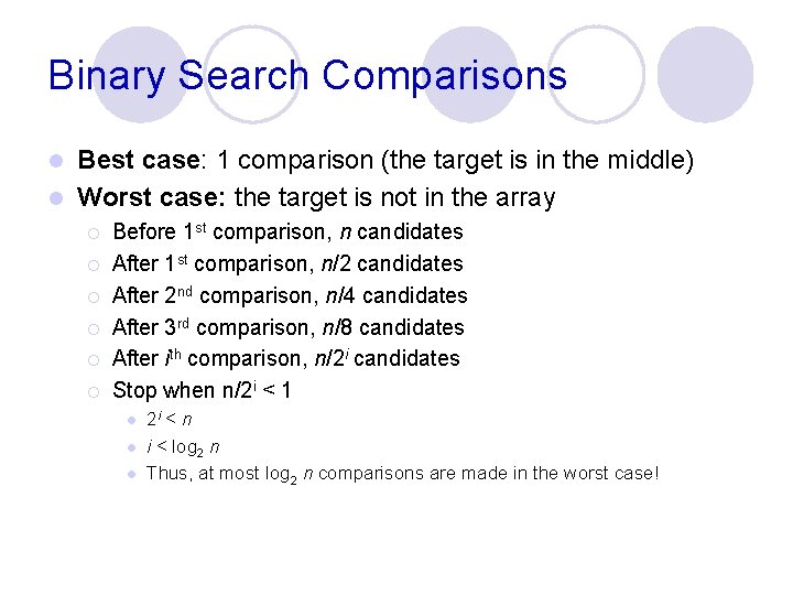
Binary Search Comparisons Best case: 1 comparison (the target is in the middle) l Worst case: the target is not in the array l ¡ ¡ ¡ Before 1 st comparison, n candidates After 1 st comparison, n/2 candidates After 2 nd comparison, n/4 candidates After 3 rd comparison, n/8 candidates After ith comparison, n/2 i candidates Stop when n/2 i < 1 l l l 2 i < n i < log 2 n Thus, at most log 2 n comparisons are made in the worst case!

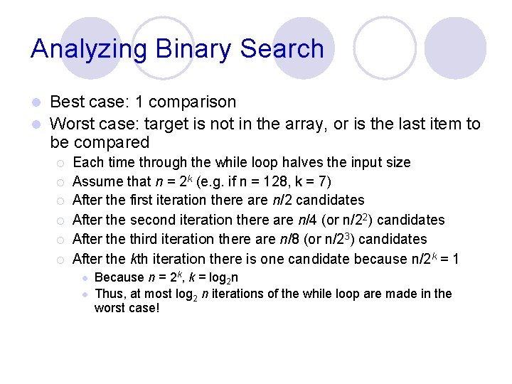
Analyzing Binary Search Best case: 1 comparison l Worst case: target is not in the array, or is the last item to be compared l ¡ ¡ ¡ Each time through the while loop halves the input size Assume that n = 2 k (e. g. if n = 128, k = 7) After the first iteration there are n/2 candidates After the second iteration there are n/4 (or n/22) candidates After the third iteration there are n/8 (or n/23) candidates After the kth iteration there is one candidate because n/2 k = 1 l l Because n = 2 k, k = log 2 n Thus, at most log 2 n iterations of the while loop are made in the worst case!

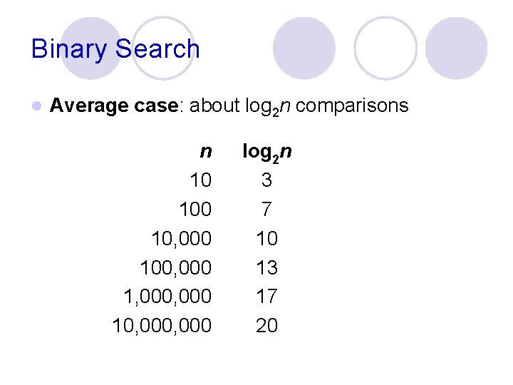
Binary Search l Average case: about log 2 n comparisons n 10 10, 000 100, 000 1, 000 10, 000 log 2 n 3 7 10 13 17 20

Selection Sort Algorithm public int selection. Sort(int[] arr){ for(int i = 0; i < arr. length-1; ++i){ int smallest = i; // Find the index of the smallest element for(int j = i + 1; j < arr. length; ++j){ if(arr[j] < arr[smallest]){ smallest = j; } } // Swap the smallest with the current item if(smallest != i){ swap(arr, smallest, i); } } }

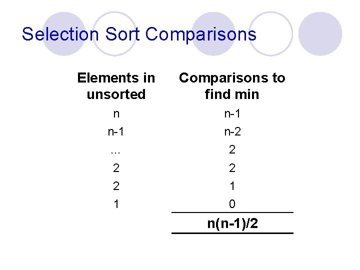
Selection Sort Comparisons Elements in unsorted Comparisons to find min n n-1 … n-1 n-2 2 1 2 1 0 n(n-1)/2

Selection Sort Analysis Makes n(n-1)/2 comparisons, regardless of the original order of the input l Makes at most n– 1 swaps (the last item must be in the correct position). l ¡ ¡ l May make less swaps depending on how the algorithm is written Can make a comparison to determine if a swap is required Total number of operations: ¡ n(n-1)/2 + n– 1

Insertion Sort Algorithm public int insertion. Sort(int[] arr){ for(int i = 1; i < arr. length; ++i){ int temp = arr[i]; int pos = i; // Shuffle up all sorted items > arr[i] while(pos > 0 && arr[pos - 1] > temp){ arr[pos] = arr[pos – 1]; pos--; } //while // Insert the current item arr[pos] = temp; } }

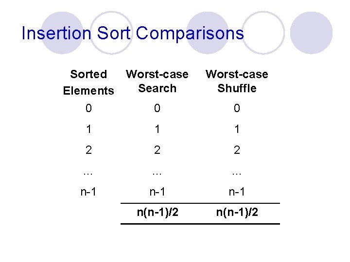
Insertion Sort Comparisons Sorted Worst-case Search Elements 0 0 Worst-case Shuffle 0 1 1 1 2 2 2 … … … n-1 n-1 n(n-1)/2

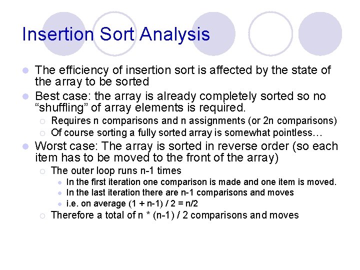
Insertion Sort Analysis The efficiency of insertion sort is affected by the state of the array to be sorted l Best case: the array is already completely sorted so no “shuffling” of array elements is required. l ¡ ¡ l Requires n comparisons and n assignments (or 2 n comparisons) Of course sorting a fully sorted array is somewhat pointless… Worst case: The array is sorted in reverse order (so each item has to be moved to the front of the array) ¡ The outer loop runs n-1 times l l l ¡ In the first iteration one comparison is made and one item is moved. In the last iteration there are n-1 comparisons and moves i. e. on average (1 + n-1) / 2 = n/2 Therefore a total of n * (n-1) / 2 comparisons and moves

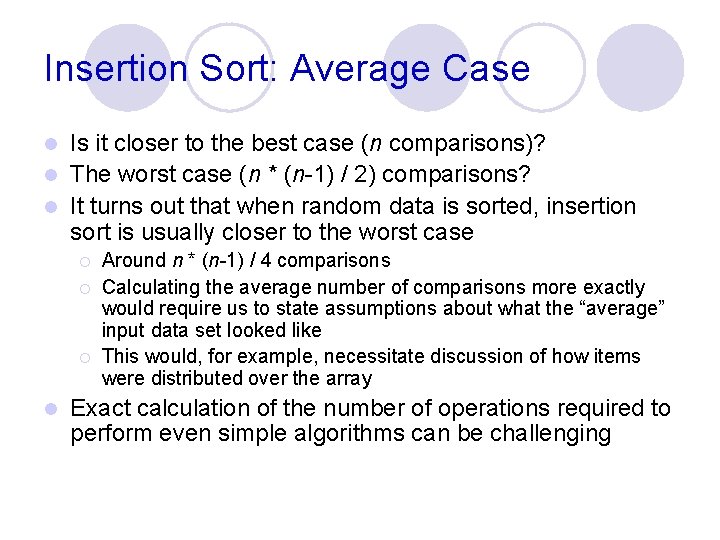
Insertion Sort: Average Case Is it closer to the best case (n comparisons)? l The worst case (n * (n-1) / 2) comparisons? l It turns out that when random data is sorted, insertion sort is usually closer to the worst case l ¡ ¡ ¡ l Around n * (n-1) / 4 comparisons Calculating the average number of comparisons more exactly would require us to state assumptions about what the “average” input data set looked like This would, for example, necessitate discussion of how items were distributed over the array Exact calculation of the number of operations required to perform even simple algorithms can be challenging

O Notation l O notation is a mathematical notation used to measure the efficiency of an algorithm ¡ l The O stands for "order of" It considers the highest order term in a function ¡ The highest order term is the term with the fastest growth rate l ¡ l e. g. n 2 grows faster than n which grows faster than log 2(n) Therefore as n (the size of the input) grows large lower order terms can be ignored It is a useful, and relatively simple measure of the efficiency of an algorithm

Growth Rate of an Algorithm In analyzing algorithms we generally want to know how they perform when the problem size (n) is large l One way of measuring this is by expressing the growth rate in the running time of an algorithm as a function of the problem size. l ¡ ¡ We’ll refer to the growth rate function of an algorithm as f(n) We expect f(n) to increase as n increases

f(n) for Selection Sort l The algorithm has an outer loop which iterates through each array position, except the last ¡ l For each index finds the smallest unsorted item ¡ ¡ ¡ l For the first item make n - 1 comparisons For the last item makes 1 comparison n/2 on average For each index swap the smallest unsorted item with the item at the current index ¡ l The loop iterates n - 1 times n – 1 times Therefore f(n) = n * (n-1) / 2 + (n – 1)

O Notation and Growth Rate l An algorithm is said to be order f(n) which is written as O(f(n)) ¡ l e. g. if an algorithm’s running time is proportional to n 2 it would be O(n 2), that is , order n 2 An algorithm, A, is O(f(n)) if: ¡ ¡ there exist constants k and n 0 such that the running time of A is k * f(n) where n n 0 e. g. if an algorithm’s running time is 3 n + 12 then the algorithm is O(n). If k is 4 and n 0 is 2 then: l 4 * n 3 n + 12 for all n 12

O Notation Properties O-notation allows lower order terms to be ignored. l Constants can be ignored (e. g. 3 in 3 * n 2 ) l Growth-rate functions can be combined l ¡ ¡ O(n) + O(m) = O(n + m) O(n) + O(n 2) = O(n + n 2), simplifies to O(n 2)

Growth Rate Functions l O(1) – constant time, the time is independent of n ¡ l O(logn) – logarithmic time, typically the log is base 2 ¡ l e. g. merge. Sort O(n 2) – quadratic time ¡ l e. g. linear search O(n*logn) ¡ l e. g. binary search O(n) – linear time ¡ l e. g. array look-up e. g. selection sort 2 n – exponential time, very slow!

Growth Rate Comparisons

Growth Rate Comparisons

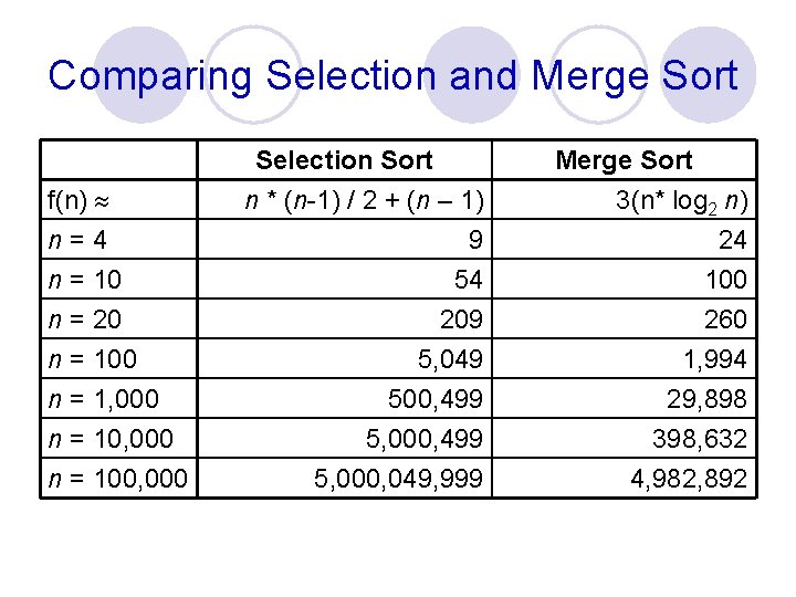
Comparing Selection and Merge Sort f(n) n=4 n = 10 n = 20 n = 100 n = 1, 000 n = 100, 000 Selection Sort n * (n-1) / 2 + (n – 1) 9 54 Merge Sort 3(n* log 2 n) 24 100 209 5, 049 500, 499 5, 000, 049, 999 260 1, 994 29, 898 398, 632 4, 982, 892

Note on Constant Time l We write O(1) to indicate something that takes a constant amount of time ¡ ¡ E. g. finding the minimum element of an ordered array takes O(1) time, because the min is either at the beginning or the end of the array Important: constants can be huge, and so in practice O(1) is not necessarily efficient --- all it tells us is that the algorithm will run at the same speed no matter the size of the input we give it

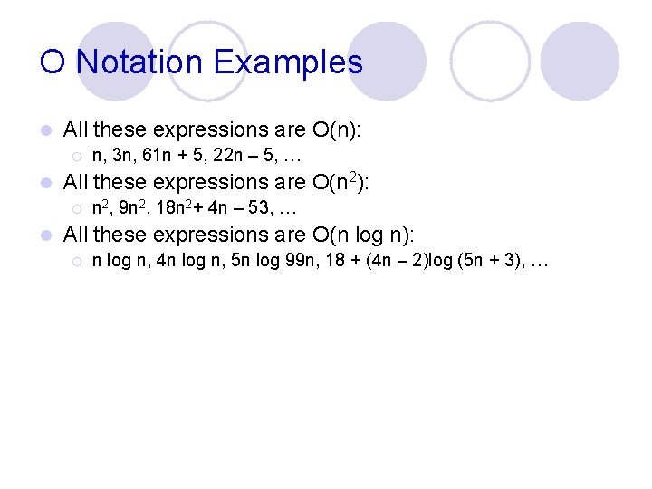
O Notation Examples l All these expressions are O(n): ¡ l All these expressions are O(n 2): ¡ l n, 3 n, 61 n + 5, 22 n – 5, … n 2, 9 n 2, 18 n 2+ 4 n – 53, … All these expressions are O(n log n): ¡ n log n, 4 n log n, 5 n log 99 n, 18 + (4 n – 2)log (5 n + 3), …