Algorithm Analysis Asymptotic notations CISC 4080 CIS Fordham

Algorithm Analysis, Asymptotic notations CISC 4080 CIS, Fordham Univ. Instructor: X. Zhang

Last class • Introduction to algorithm analysis: fibonacci seq calculation • counting number of “computer steps” • recursive formula for running time of recursive algorithm 2

Outline • Review of algorithm analysis • counting number of “computer steps” (or representative operations) • recursive formula for running time of recursive algorithm • math help: math. induction • Asymptotic notations • Algorithm running time classes: P, NP 3

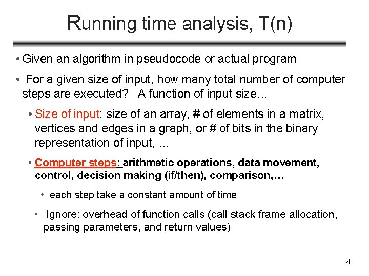
Running time analysis, T(n) • Given an algorithm in pseudocode or actual program • For a given size of input, how many total number of computer steps are executed? A function of input size… • Size of input: size of an array, # of elements in a matrix, vertices and edges in a graph, or # of bits in the binary representation of input, … • Computer steps: arithmetic operations, data movement, control, decision making (if/then), comparison, … • each step take a constant amount of time • Ignore: overhead of function calls (call stack frame allocation, passing parameters, and return values) 4

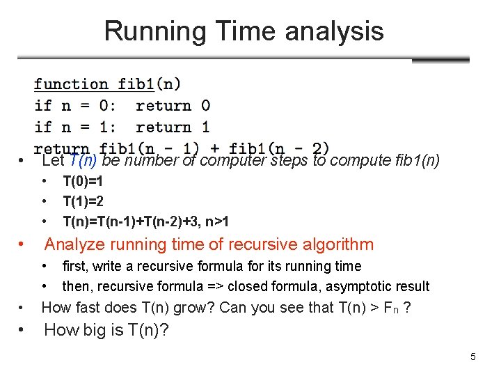
Running Time analysis • Let T(n) be number of computer steps to compute fib 1(n) • • T(0)=1 T(1)=2 T(n)=T(n-1)+T(n-2)+3, n>1 Analyze running time of recursive algorithm • • first, write a recursive formula for its running time then, recursive formula => closed formula, asymptotic result • How fast does T(n) grow? Can you see that T(n) > Fn ? • How big is T(n)? 5

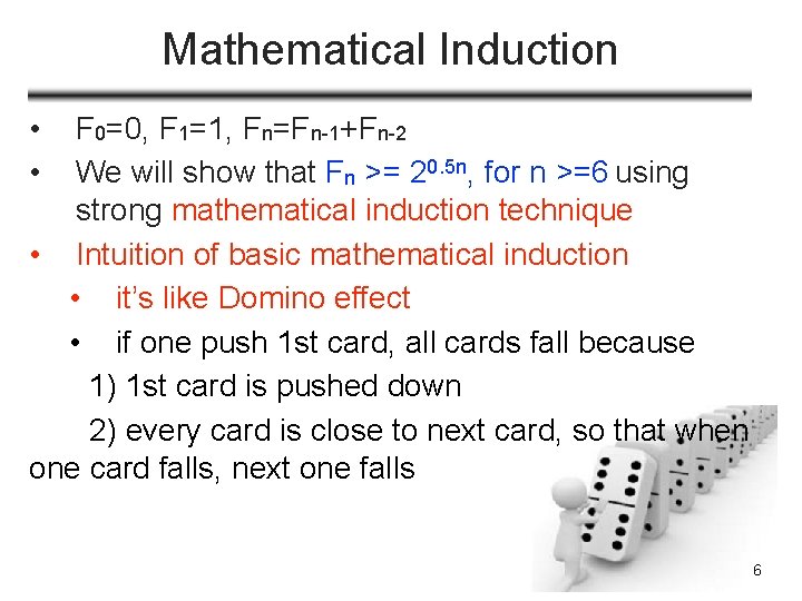
Mathematical Induction • • F 0=0, F 1=1, Fn=Fn-1+Fn-2 We will show that Fn >= 20. 5 n, for n >=6 using strong mathematical induction technique • Intuition of basic mathematical induction • it’s like Domino effect • if one push 1 st card, all cards fall because 1) 1 st card is pushed down 2) every card is close to next card, so that when one card falls, next one falls 6

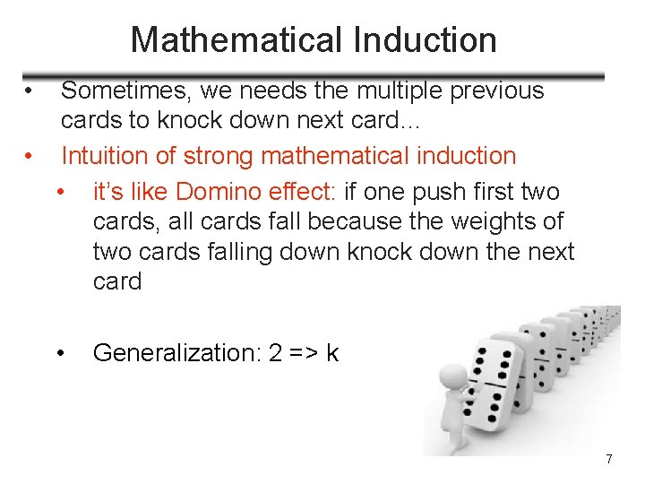
Mathematical Induction • Sometimes, we needs the multiple previous cards to knock down next card… • Intuition of strong mathematical induction • it’s like Domino effect: if one push first two cards, all cards fall because the weights of two cards falling down knock down the next card • Generalization: 2 => k 7

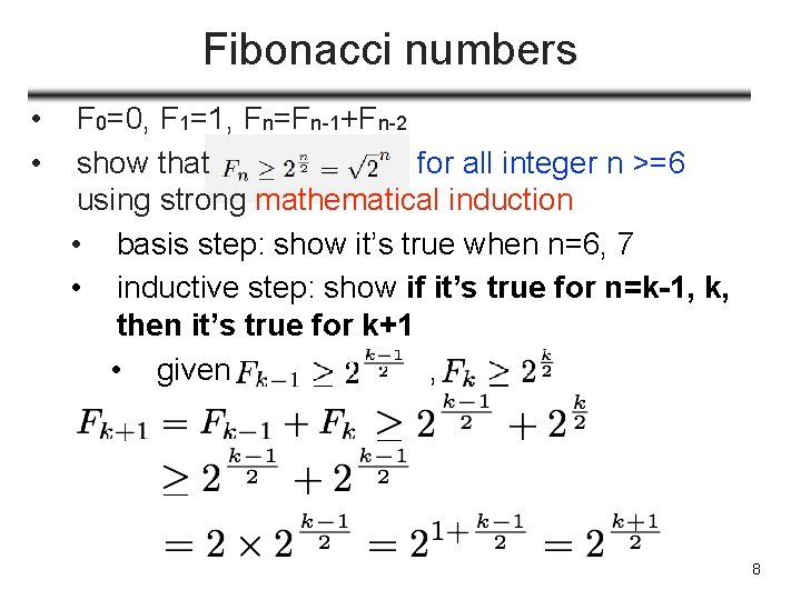
Fibonacci numbers • • F 0=0, F 1=1, Fn=Fn-1+Fn-2 show that for all integer n >=6 using strong mathematical induction • basis step: show it’s true when n=6, 7 • inductive step: show if it’s true for n=k-1, k, then it’s true for k+1 • given , 8

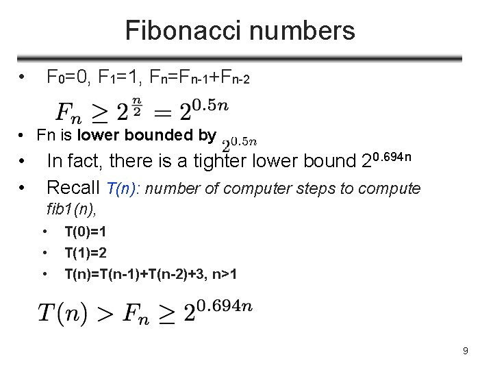
Fibonacci numbers • F 0=0, F 1=1, Fn=Fn-1+Fn-2 • Fn is lower bounded by • • In fact, there is a tighter lower bound 20. 694 n Recall T(n): number of computer steps to compute fib 1(n), • • • T(0)=1 T(1)=2 T(n)=T(n-1)+T(n-2)+3, n>1 9

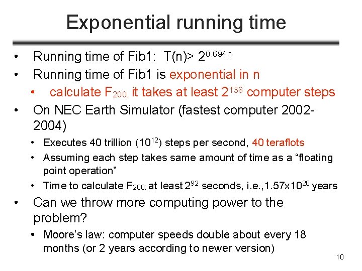
Exponential running time • • Running time of Fib 1: T(n)> 20. 694 n Running time of Fib 1 is exponential in n • calculate F 200, it takes at least 2138 computer steps • On NEC Earth Simulator (fastest computer 20022004) • Executes 40 trillion (1012) steps per second, 40 teraflots • Assuming each step takes same amount of time as a “floating point operation” • Time to calculate F 200: at least 292 seconds, i. e. , 1. 57 x 1020 years • Can we throw more computing power to the problem? • Moore’s law: computer speeds double about every 18 months (or 2 years according to newer version) 10

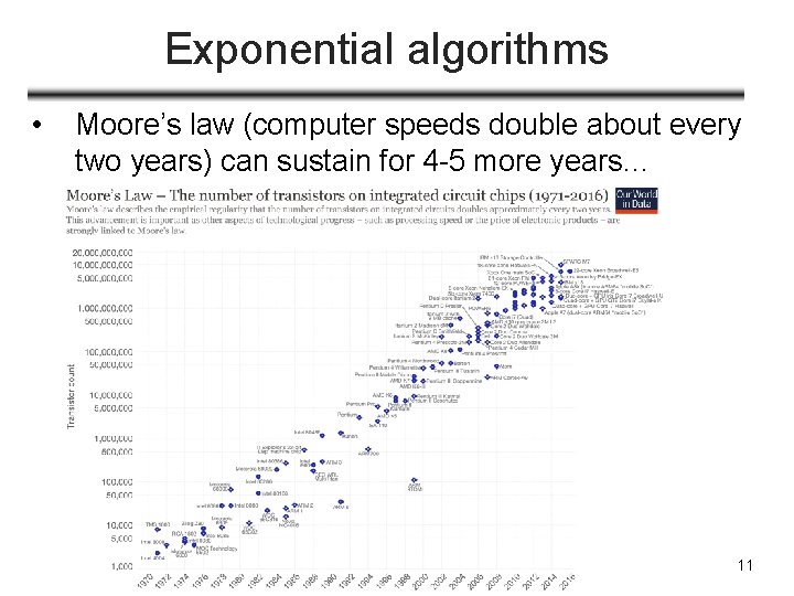
Exponential algorithms • Moore’s law (computer speeds double about every two years) can sustain for 4 -5 more years… 11

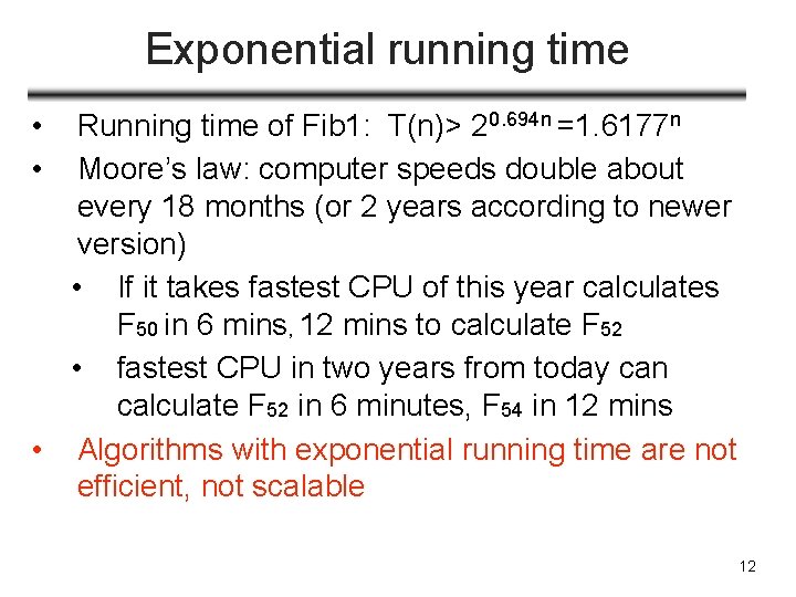
Exponential running time • • Running time of Fib 1: T(n)> 20. 694 n =1. 6177 n Moore’s law: computer speeds double about every 18 months (or 2 years according to newer version) • If it takes fastest CPU of this year calculates F 50 in 6 mins, 12 mins to calculate F 52 • fastest CPU in two years from today can calculate F 52 in 6 minutes, F 54 in 12 mins • Algorithms with exponential running time are not efficient, not scalable 12

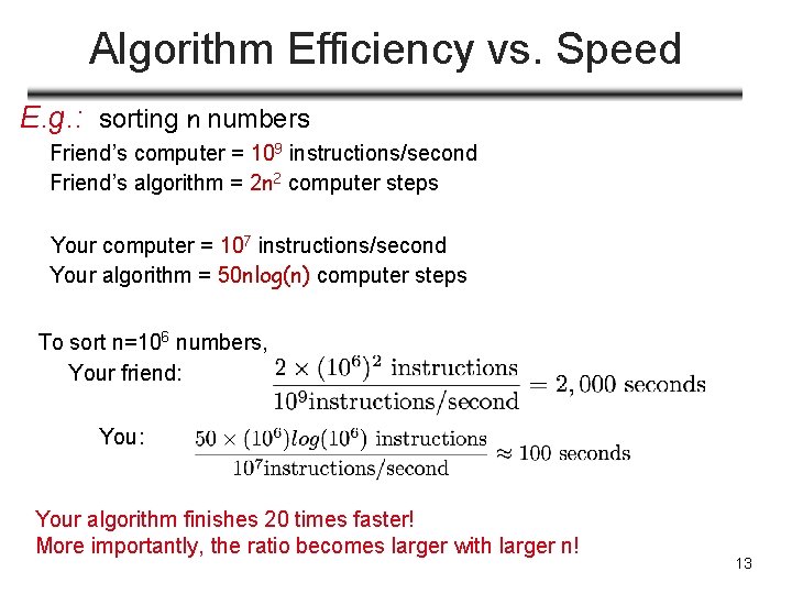
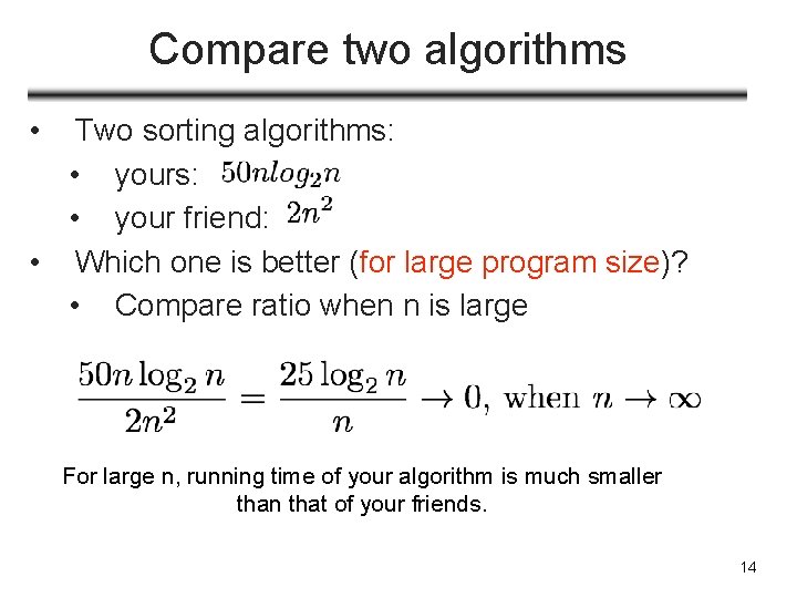
Algorithm Efficiency vs. Speed E. g. : sorting n numbers Friend’s computer = 109 instructions/second Friend’s algorithm = 2 n 2 computer steps Your computer = 107 instructions/second Your algorithm = 50 nlog(n) computer steps To sort n=106 numbers, Your friend: You: Your algorithm finishes 20 times faster! More importantly, the ratio becomes larger with larger n! 13

Compare two algorithms • Two sorting algorithms: • your friend: • Which one is better (for large program size)? • Compare ratio when n is large For large n, running time of your algorithm is much smaller than that of your friends. 14

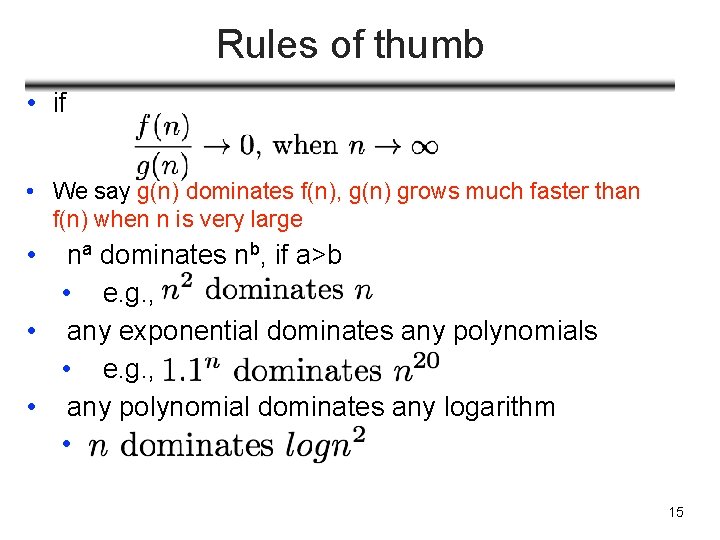
Rules of thumb • if • We say g(n) dominates f(n), g(n) grows much faster than f(n) when n is very large • na dominates nb, if a>b • e. g. , • any exponential dominates any polynomials • e. g. , • any polynomial dominates any logarithm • 15

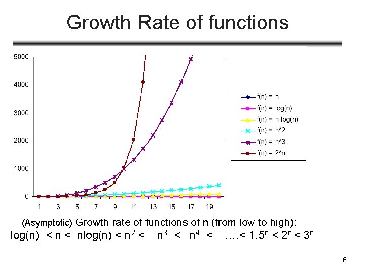
Growth Rate of functions • e. g. , f(x)=2 x: asymptotic growth rate is 2 • : very big! (Asymptotic) Growth rate of functions of n (from low to high): log(n) < nlog(n) < n 2 < n 3 < n 4 < …. < 1. 5 n < 2 n < 3 n 16

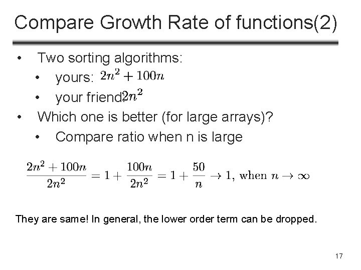
Compare Growth Rate of functions(2) • Two sorting algorithms: • your friend: • Which one is better (for large arrays)? • Compare ratio when n is large They are same! In general, the lower order term can be dropped. 17

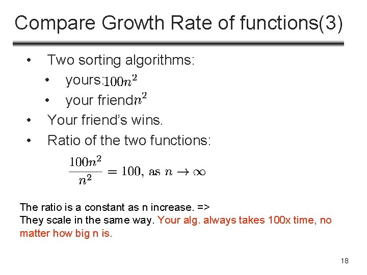
Compare Growth Rate of functions(3) • Two sorting algorithms: • your friend: • Your friend’s wins. • Ratio of the two functions: The ratio is a constant as n increase. => They scale in the same way. Your alg. always takes 100 x time, no matter how big n is. 18

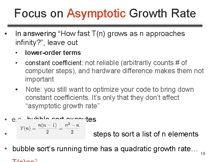
Focus on Asymptotic Growth Rate • In answering “How fast T(n) grows as n approaches infinity? ”, leave out • • lower-order terms • Note: you still want to optimize your code to bring down constant coefficients. It’s only that they don’t affect “asymptotic growth rate” constant coefficient: not reliable (arbitrarily counts # of computer steps), and hardware difference makes them not important • e. g. , bubble sort executes • steps to sort a list of n elements • bubble sort’s running time has a quadratic growth rate… 19

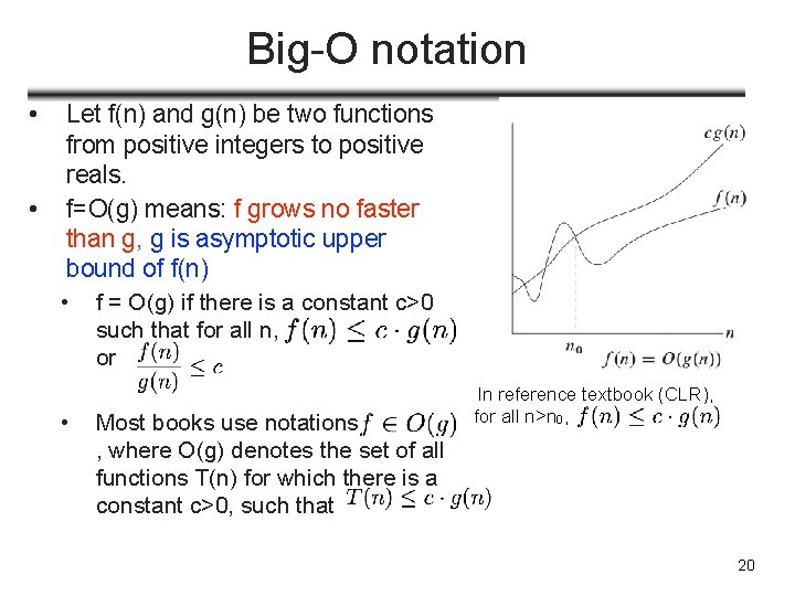
Big-O notation • • Let f(n) and g(n) be two functions from positive integers to positive reals. f=O(g) means: f grows no faster than g, g is asymptotic upper bound of f(n) • • f = O(g) if there is a constant c>0 such that for all n, or Most books use notations , where O(g) denotes the set of all functions T(n) for which there is a constant c>0, such that In reference textbook (CLR), for all n>n 0, 20

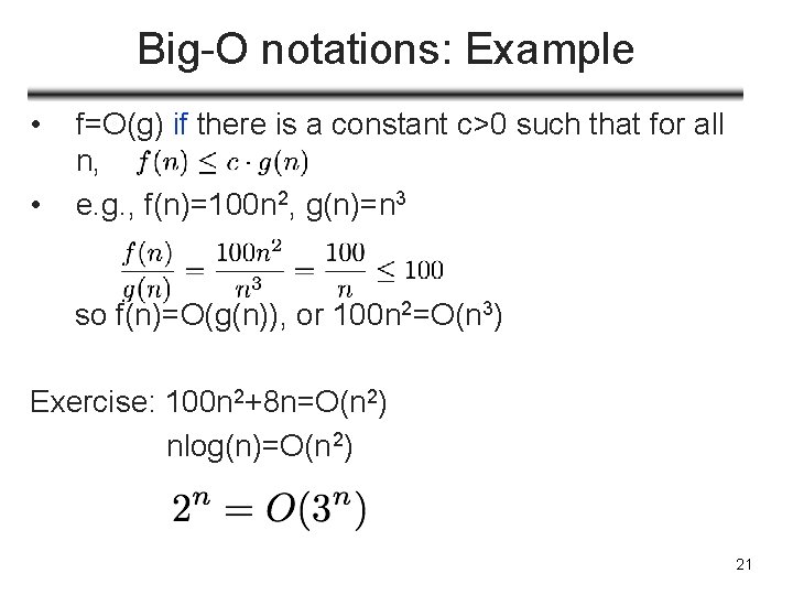
Big-O notations: Example • • f=O(g) if there is a constant c>0 such that for all n, e. g. , f(n)=100 n 2, g(n)=n 3 so f(n)=O(g(n)), or 100 n 2=O(n 3) Exercise: 100 n 2+8 n=O(n 2) nlog(n)=O(n 2) 21

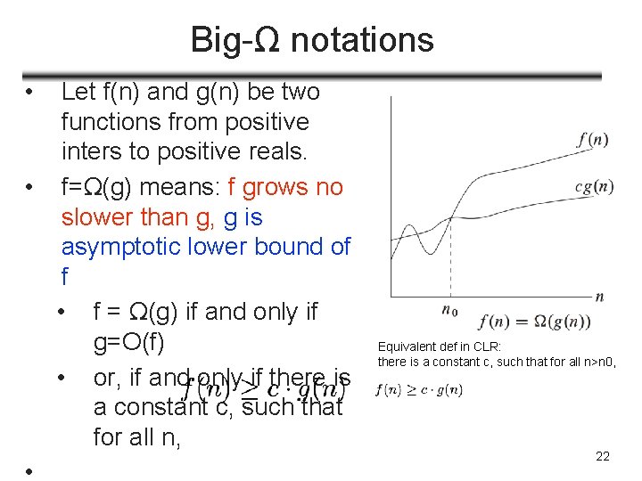
Big-Ω notations • Let f(n) and g(n) be two functions from positive inters to positive reals. • f=Ω(g) means: f grows no slower than g, g is asymptotic lower bound of f • f = Ω(g) if and only if g=O(f) • or, if and only if there is a constant c, such that for all n, • Equivalent def in CLR: there is a constant c, such that for all n>n 0, 22

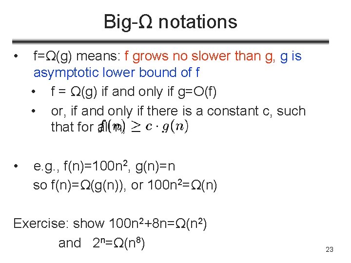
Big-Ω notations • f=Ω(g) means: f grows no slower than g, g is asymptotic lower bound of f • f = Ω(g) if and only if g=O(f) • or, if and only if there is a constant c, such that for all n, • e. g. , f(n)=100 n 2, g(n)=n so f(n)=Ω(g(n)), or 100 n 2=Ω(n) Exercise: show 100 n 2+8 n=Ω(n 2) and 2 n=Ω(n 8) 23

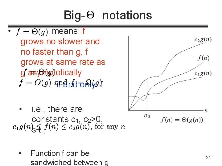
Big • notations means: f grows no slower and no faster than g, f grows at same rate as g asymptotically • if and only if • i. e. , there are constants c 1, c 2>0, s. t. , • Function f can be sandwiched between g 24

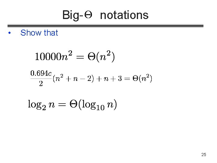
Big • notations Show that 25

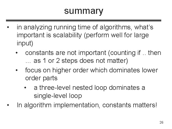
summary • in analyzing running time of algorithms, what’s important is scalability (perform well for large input) • constants are not important (counting if. . then … as 1 or 2 steps does not matter) • focus on higher order which dominates lower order parts • a three-level nested loop dominates a single-level loop • In algorithm implementation, constants matters! 26

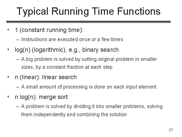
Typical Running Time Functions • 1 (constant running time): – Instructions are executed once or a few times • log(n) (logarithmic), e. g. , binary search – A big problem is solved by cutting original problem in smaller sizes, by a constant fraction at each step • n (linear): linear search – A small amount of processing is done on each input element • n log(n): merge sort – A problem is solved by dividing it into smaller problems, solving them independently and combining the solution 27

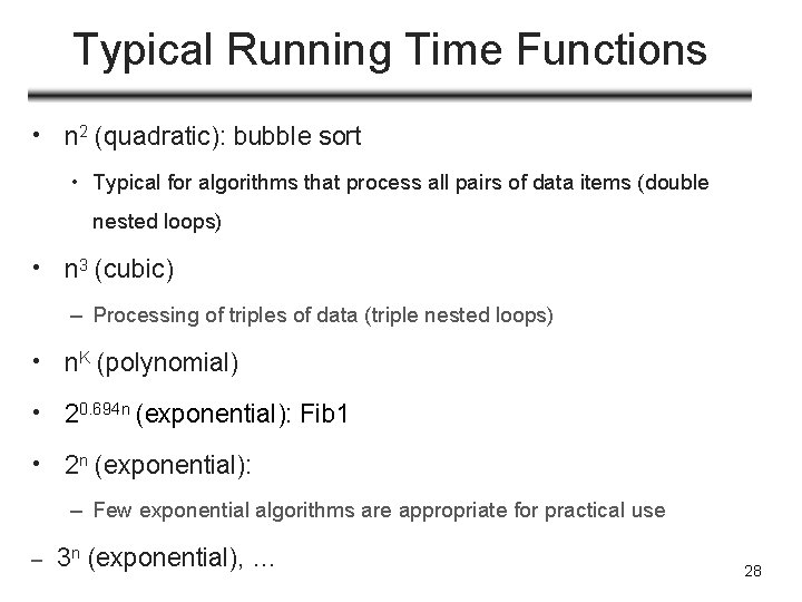
Typical Running Time Functions • n 2 (quadratic): bubble sort • Typical for algorithms that process all pairs of data items (double nested loops) • n 3 (cubic) – Processing of triples of data (triple nested loops) • n. K (polynomial) • 20. 694 n (exponential): Fib 1 • 2 n (exponential): – Few exponential algorithms are appropriate for practical use – 3 n (exponential), … 28

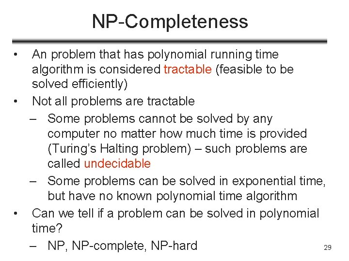
NP-Completeness • An problem that has polynomial running time algorithm is considered tractable (feasible to be solved efficiently) • Not all problems are tractable – Some problems cannot be solved by any computer no matter how much time is provided (Turing’s Halting problem) – such problems are called undecidable – Some problems can be solved in exponential time, but have no known polynomial time algorithm • Can we tell if a problem can be solved in polynomial time? – NP, NP-complete, NP-hard 29

Summary • algorithm running time analysis • start with running time function, expressing number of computer steps in terms of input size • Focus on very large problem size, i. e. , asymptotic running time • big-O notations => focus on dominating terms in running time function • Constant, linear, polynomial, exponential time algorithms … • NP, NP complete problem 30

Coming up? • Algorithm analysis is only one aspect of the class • We will look at different algorithms design paradigm, using problems from a wide range of domain (number, encryption, sorting, searching, graph, …) • First, Divide and Conquer algorithms and Master Theorem 31

Readings • Chapter 0, DPV • Chapter 3, CLR 32