Algorithm Analysis Algorithms that are equally correct can

Algorithm Analysis § Algorithms that are equally correct can vary in their utilization of computational resources § time and memory § a slow program it is likely not to be used § a program that demands too much memory may not be executable on the machines that are available E. G. M. Petrakis Algorithm Analysis 1

Memory - Time § It is important to be able to predict how an algorithm behaves under a range of possible conditions § different inputs § The emphasis is on the time rather than on the space efficiency § memory is cheap! E. G. M. Petrakis Algorithm Analysis 2

Running Time § The time to solve a problem increases with the size of the input § measure the rate at which the time increases § e. g. , linearly, quadratically, exponentially § This measure focuses on intrinsic characteristics of the algorithm rather than incidental factors § e. g. , computer speed, coding tricks, optimizations, quality of compiler E. G. M. Petrakis Algorithm Analysis 3

Additional Consideration § Sometimes, simple but less efficient algorithms are preferred over more efficient ones § the more efficient algorithms are not always easy to implement § the program is to be changed soon § time may not be critical § the program will run only few times (e. g. , once a year) § the size of the input is always very small E. G. M. Petrakis Algorithm Analysis 4

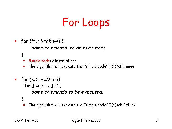
For Loops § for (i=1; i<=N; i++) { some commands to be executed; } § Simple code: c instructions § The algorithm will execute the “simple code” T(n)=c. N times § for (i=1; i<=N; i++) for (j=1; j<= N; j++) { some commands to be executed; } § The algorithm will execute the “simple code” T(n)=c. N 2 times E. G. M. Petrakis Algorithm Analysis 5

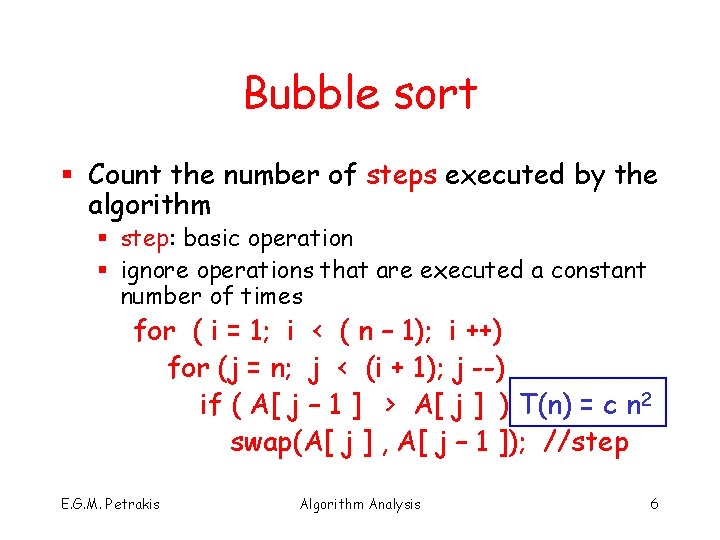
Bubble sort § Count the number of steps executed by the algorithm § step: basic operation § ignore operations that are executed a constant number of times for ( i = 1; i < ( n – 1); i ++) for (j = n; j < (i + 1); j --) if ( A[ j – 1 ] > A[ j ] ) T(n) = c n 2 swap(A[ j ] , A[ j – 1 ]); //step E. G. M. Petrakis Algorithm Analysis 6

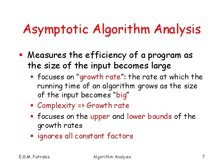
Asymptotic Algorithm Analysis § Measures the efficiency of a program as the size of the input becomes large § focuses on “growth rate”: the rate at which the running time of an algorithm grows as the size of the input becomes “big” § Complexity => Growth rate § focuses on the upper and lower bounds of the growth rates § ignores all constant factors E. G. M. Petrakis Algorithm Analysis 7

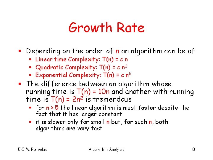
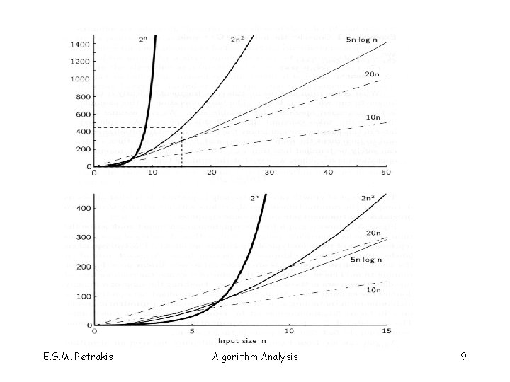
Growth Rate § Depending on the order of n an algorithm can be of § Linear time Complexity: T(n) = c n § Quadratic Complexity: T(n) = c n 2 § Exponential Complexity: T(n) = c nk § The difference between an algorithm whose running time is T(n) = 10 n and another with running time is T(n) = 2 n 2 is tremendous § for n > 5 the linear algorithm is must faster despite the fact that it has larger constant § it is slower only for small n but, for such n, both algorithms are very fast E. G. M. Petrakis Algorithm Analysis 8

E. G. M. Petrakis Algorithm Analysis 9

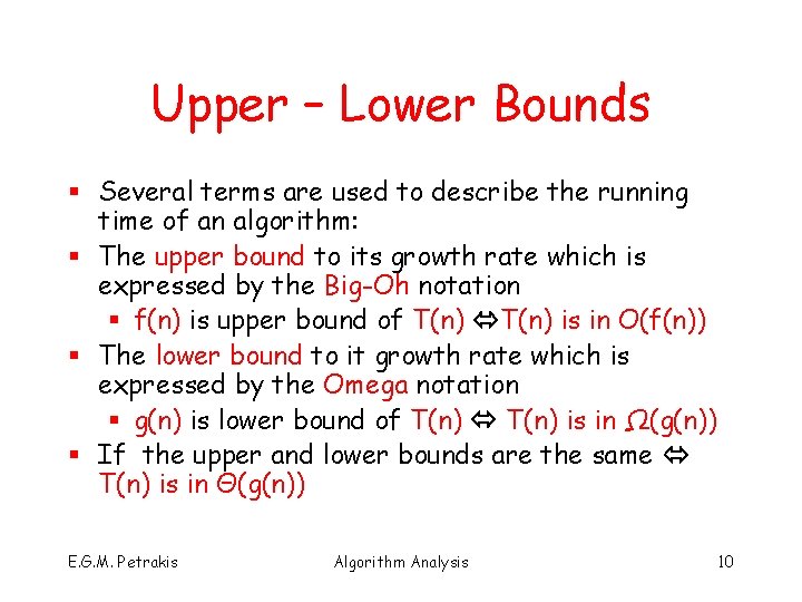
Upper – Lower Bounds § Several terms are used to describe the running time of an algorithm: § The upper bound to its growth rate which is expressed by the Big-Oh notation § f(n) is upper bound of T(n) is in O(f(n)) § The lower bound to it growth rate which is expressed by the Omega notation § g(n) is lower bound of T(n) is in Ω(g(n)) § If the upper and lower bounds are the same T(n) is in Θ(g(n)) E. G. M. Petrakis Algorithm Analysis 10

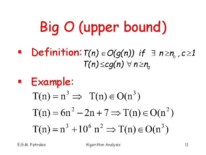
Big O (upper bound) § Definition: § Example: E. G. M. Petrakis Algorithm Analysis 11

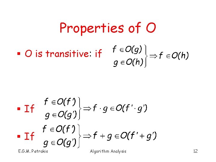
Properties of O § O is transitive: if § If E. G. M. Petrakis Algorithm Analysis 12

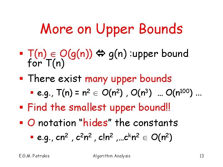
More on Upper Bounds § T(n) O(g(n)) g(n) : upper bound for T(n) § There exist many upper bounds § e. g. , T(n) = n 2 O(n 2) , O(n 3) … O(n 100). . . § Find the smallest upper bound!! § O notation “hides” the constants § e. g. , cn 2 , c 2 n 2 , c!n 2 , …ckn 2 O(n 2) E. G. M. Petrakis Algorithm Analysis 13

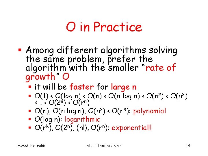
O in Practice § Among different algorithms solving the same problem, prefer the algorithm with the smaller “rate of growth” O § it will be faster for large n § Ο(1) < Ο(log n) < Ο(n 2) < Ο(n 3) < …< Ο(2 n) < O(nn) § Ο(n), Ο(n log n), Ο(n 2) < Ο(n 3): polynomial § Ο(log n): logarithmic § O(nk), O(2 n), (n!), O(nn): exponential!! E. G. M. Petrakis Algorithm Analysis 14

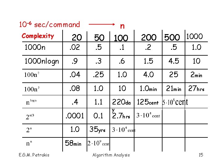
10 -6 sec/command Complexity 1000 nlogn 20 50 n 100 . 9 . 3 . 04 . 02 . 5 . 1 200 500 1000. 2 . 5 1. 0 . 6 1. 5 4. 5 10 . 25 1. 0 4. 0 25 2 min . 08 1. 0 10 1. 0 min . 4 1. 1 220 da 125 cent . 0001 0. 1 2. 7 hrs 1. 0 35 yrs 21 min 27 hrs y 58 min E. G. M. Petrakis Algorithm Analysis 15

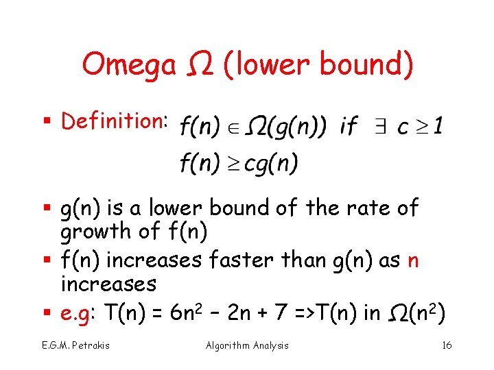
Omega Ω (lower bound) § Definition: § g(n) is a lower bound of the rate of growth of f(n) § f(n) increases faster than g(n) as n increases § e. g: T(n) = 6 n 2 – 2 n + 7 =>T(n) in Ω(n 2) E. G. M. Petrakis Algorithm Analysis 16

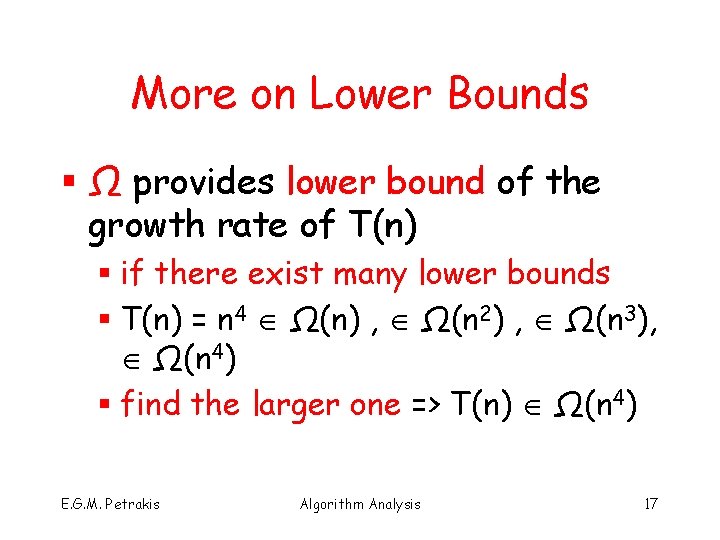
More on Lower Bounds § Ω provides lower bound of the growth rate of T(n) § if there exist many lower bounds § T(n) = n 4 Ω(n) , Ω(n 2) , Ω(n 3), Ω(n 4) § find the larger one => T(n) Ω(n 4) E. G. M. Petrakis Algorithm Analysis 17

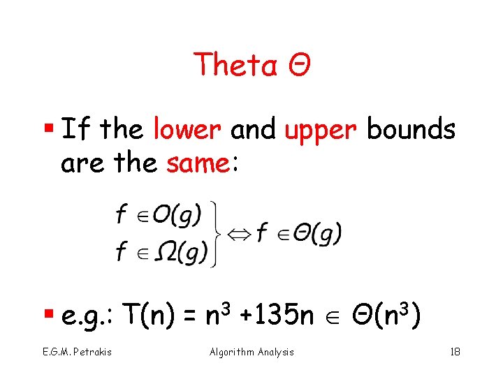
Thetα Θ § If the lower and upper bounds are the same: § e. g. : T(n) = n 3 +135 n Θ(n 3) E. G. M. Petrakis Algorithm Analysis 18

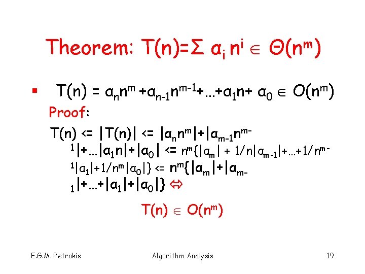
Theorem: T(n)=Σ αi ni Θ(nm) § T(n) = αnnm +αn-1 nm-1+…+α 1 n+ α 0 O(nm) Proof: T(n) <= |T(n)| <= |αnnm|+|αm-1 nm 1|+…|α n|+|α | <= nm{|α | + 1/n|α |+…+1/nmm m-1 1 0 1|α |+1/nm|α |} <= nm{|α |+|α 1 0 m m 1|+…+|α 1|+|α 0|} T(n) O(nm) E. G. M. Petrakis Algorithm Analysis 19

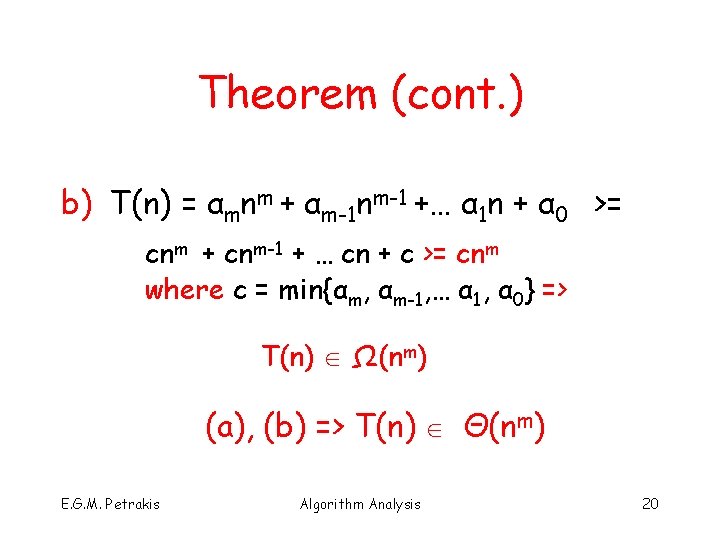
Theorem (cont. ) b) T(n) = αmnm + αm-1 nm-1 +… α 1 n + α 0 >= cnm + cnm-1 + … cn + c >= cnm where c = min{αm, αm-1, … α 1, α 0} => T(n) Ω(nm) (a), (b) => Τ(n) Θ(nm) E. G. M. Petrakis Algorithm Analysis 20

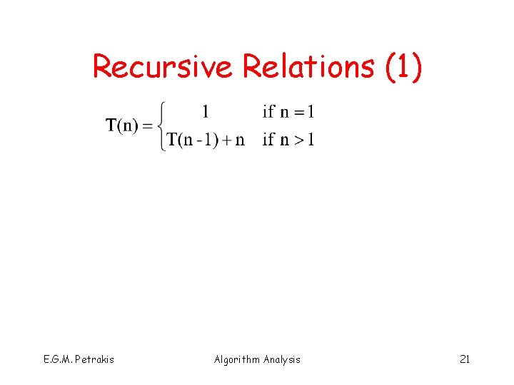
Recursive Relations (1) E. G. M. Petrakis Algorithm Analysis 21

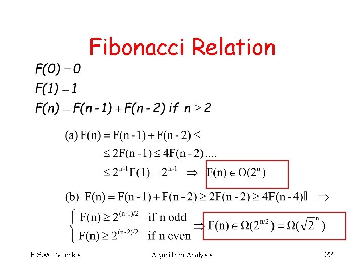
Fibonacci Relation E. G. M. Petrakis Algorithm Analysis 22

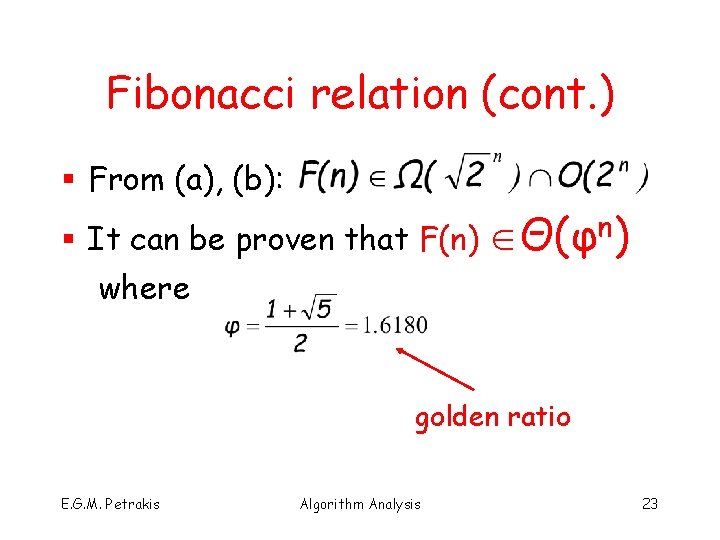
Fibonacci relation (cont. ) § From (a), (b): § It can be proven that F(n) Θ(φn) where golden ratio E. G. M. Petrakis Algorithm Analysis 23

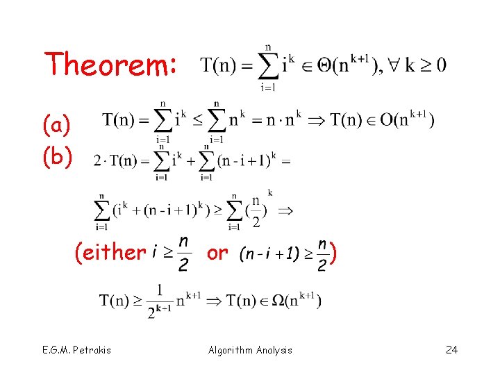
Theorem: (a) (b) (either E. G. M. Petrakis or Algorithm Analysis ) 24

Binary Search int BSearch(int table[a. . b], key, n) { if (a > b) return (– 1) ; int middle = (a + b)/2 ; if (T[middle] == key) return (middle); else if ( key < T[middle] ) return BSearch(T[a. . middle – 1], key); else return BSearch(T[middle + 1. . b], key); } E. G. M. Petrakis Algorithm Analysis 25

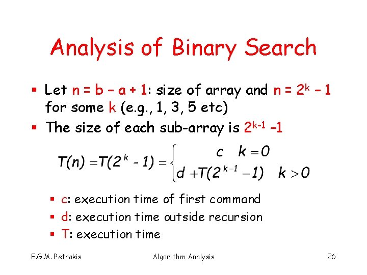
Analysis of Binary Search § Let n = b – a + 1: size of array and n = 2 k – 1 for some k (e. g. , 1, 3, 5 etc) § The size of each sub-array is 2 k-1 – 1 § c: execution time of first command § d: execution time outside recursion § T: execution time E. G. M. Petrakis Algorithm Analysis 26

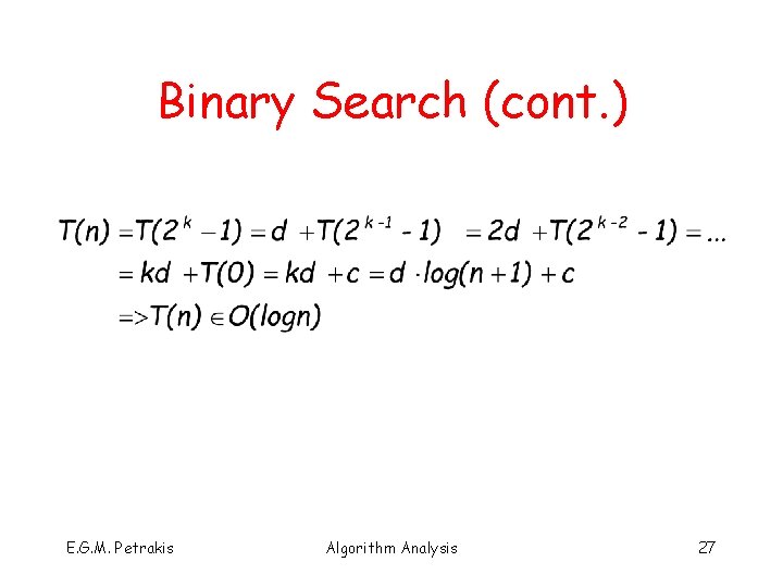
Binary Search (cont. ) E. G. M. Petrakis Algorithm Analysis 27

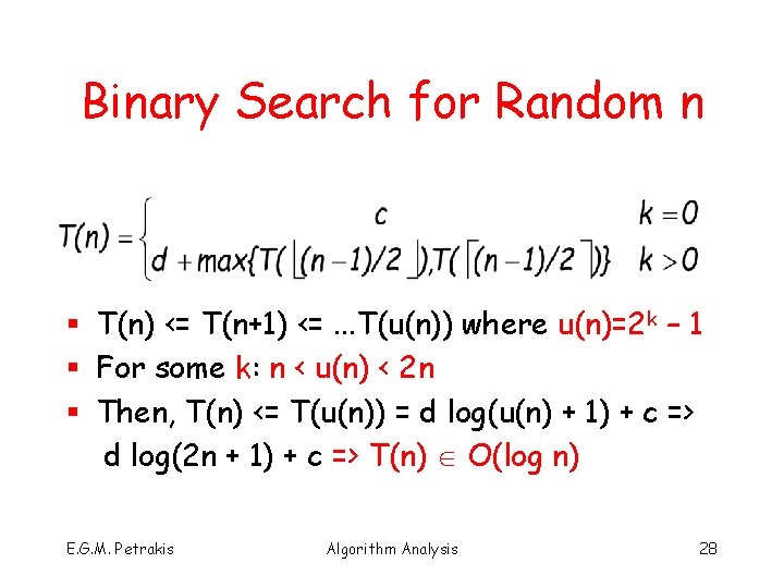
Binary Search for Random n § T(n) <= T(n+1) <=. . . T(u(n)) where u(n)=2 k – 1 § For some k: n < u(n) < 2 n § Then, T(n) <= T(u(n)) = d log(u(n) + 1) + c => d log(2 n + 1) + c => T(n) O(log n) E. G. M. Petrakis Algorithm Analysis 28

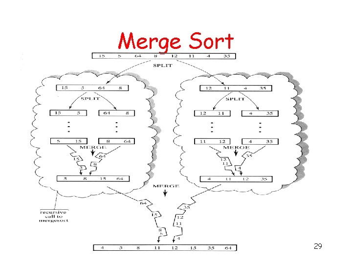
Merge Sort 29

Analysis of Merge sort [57] [48] [37] [12] [92] [86] [33] [25 57] [37 48] [12 92] [33 86] [25 37 48 57] [12 33 86 92] [12 25 33 37 48 57 86 92] log 2 n merges [25] n steps per merge, log 2 n steps/merge => O(n log 2 n) E. G. M. Petrakis Algorithm Analysis 30

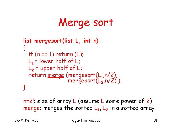
Merge sort list mergesort(list L, int n) { if (n == 1) return (L); L 1 = lower half of L; L 2 = upper half of L; return merge (mergesort(L 1, n/2), mergesort(L 2, n/2) ); } n=2 i: size of array L (assume L some power of 2) merge: merges the sorted L 1, L 2 in a sorted array E. G. M. Petrakis Algorithm Analysis 31

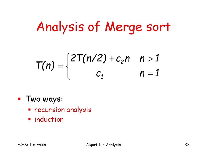
Analysis of Merge sort § Two ways: § recursion analysis § induction E. G. M. Petrakis Algorithm Analysis 32

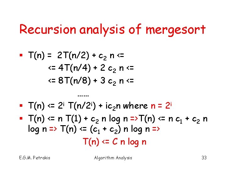
Recursion analysis of mergesort § T(n) = 2 T(n/2) + c 2 n <= <= 4 T(n/4) + 2 c 2 n <= <= 8 T(n/8) + 3 c 2 n <= …… § T(n) <= 2 i T(n/2 i) + ic 2 n where n = 2 i § T(n) <= n T(1) + c 2 n log n =>T(n) <= n c 1 + c 2 n log n => T(n) <= (c 1 + c 2) n log n => T(n) <= C n log n E. G. M. Petrakis Algorithm Analysis 33

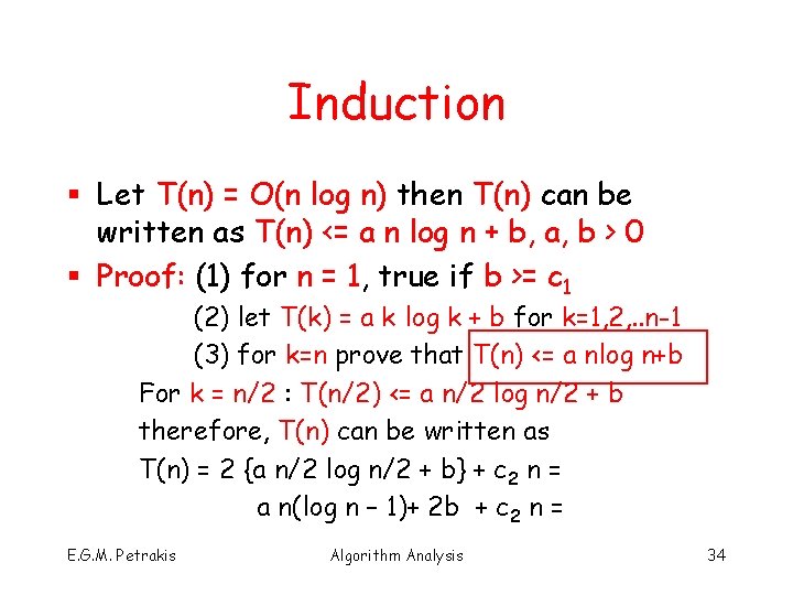
Induction § Let T(n) = O(n log n) then T(n) can be written as T(n) <= a n log n + b, a, b > 0 § Proof: (1) for n = 1, true if b >= c 1 (2) let T(k) = a k log k + b for k=1, 2, . . n-1 (3) for k=n prove that T(n) <= a nlog n+b For k = n/2 : T(n/2) <= a n/2 log n/2 + b therefore, T(n) can be written as T(n) = 2 {a n/2 log n/2 + b} + c 2 n = a n(log n – 1)+ 2 b + c 2 n = E. G. M. Petrakis Algorithm Analysis 34

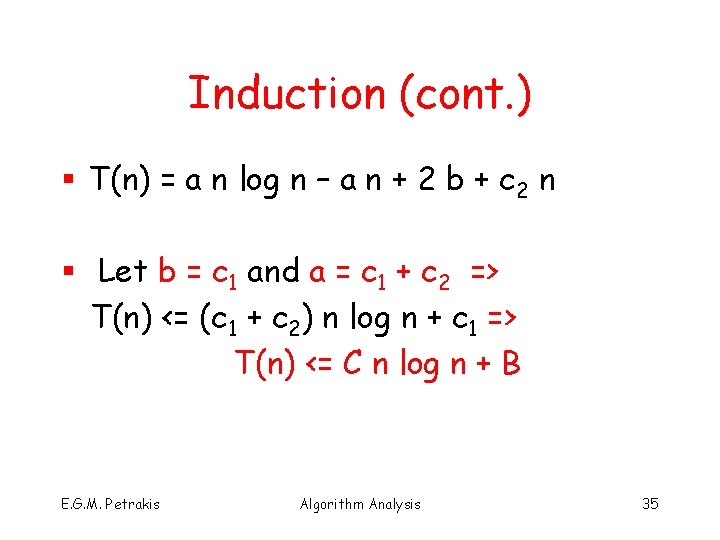
Induction (cont. ) § T(n) = a n log n – a n + 2 b + c 2 n § Let b = c 1 and a = c 1 + c 2 => T(n) <= (c 1 + c 2) n log n + c 1 => T(n) <= C n log n + B E. G. M. Petrakis Algorithm Analysis 35

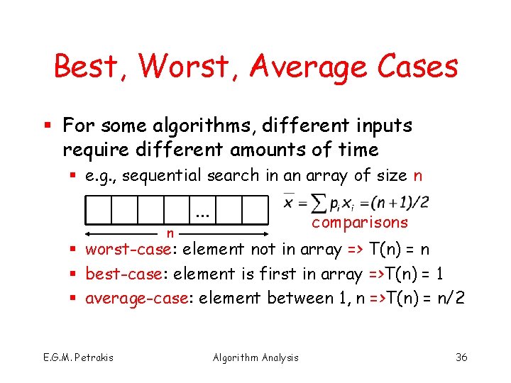
Best, Worst, Average Cases § For some algorithms, different inputs require different amounts of time § e. g. , sequential search in an array of size n n . . . comparisons § worst-case: element not in array => T(n) = n § best-case: element is first in array =>T(n) = 1 § average-case: element between 1, n =>T(n) = n/2 E. G. M. Petrakis Algorithm Analysis 36

Comparison § The best-case is not representative § happens only rarely § useful when it has high probability § The worst-case is very useful: § the algorithm performs at least that well § very important for real-time applications § The average-case represents the typical behavior of the algorithm § not always possible § knowledge about data distribution is necessary E. G. M. Petrakis Algorithm Analysis 37