Algorithm Analysis Algorithm Complexity Correctness is Not Enough

Algorithm Analysis (Algorithm Complexity)

Correctness is Not Enough • It isn’t sufficient that our algorithms perform the required tasks. • We want them to do so efficiently, making the best use of – Space (Storage) – Time (How long will it take, Number of instructions)

Time and Space • Time – Instructions take time. – How fast does the algorithm perform? – What affects its runtime? • Space – Data structures take space. – What kind of data structures can be used? – How does the choice of data structure affect the runtime?

Time vs. Space Very often, we can trade space for time: For example: maintain a collection of students’ with SSN information. – Use an array of a billion elements and have immediate access (better time) – Use an array of 100 elements and have to search (better space)

The Right Balance The best solution uses a reasonable mix of space and time. – Select effective data structures to represent your data model. – Utilize efficient methods on these data structures.

Measuring the Growth of Work While it is possible to measure the work done by an algorithm for a given set of input, we need a way to: – Measure the rate of growth of an algorithm based upon the size of the input – Compare algorithms to determine which is better for the situation

Worst-Case Analysis • Worst case running time – Obtain bound on largest possible running time of algorithm on input of a given size N – Generally captures efficiency in practice We will focus on the Worst-Case when analyzing algorithms 7

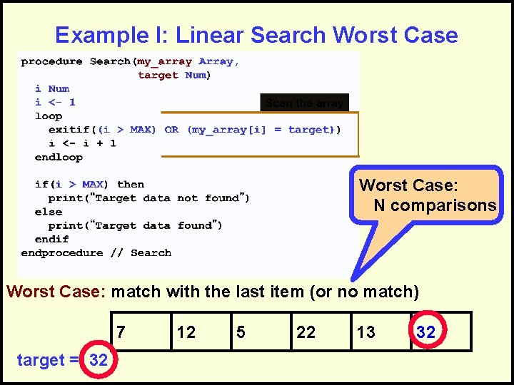
Example I: Linear Search Worst Case: N comparisons Worst Case: match with the last item (or no match) 7 target = 32 12 5 22 13 32

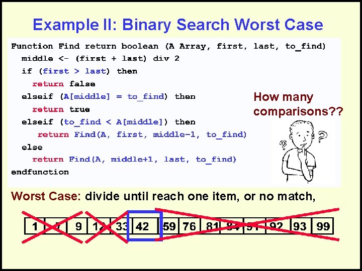
Example II: Binary Search Worst Case How many comparisons? ? Worst Case: divide until reach one item, or no match,

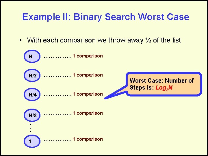
Example II: Binary Search Worst Case • With each comparison we throw away ½ of the list N ………… 1 comparison N/2 ………… 1 comparison N/4 ………… 1 comparison N/8 ………… 1 comparison . . . 1 ………… 1 comparison Worst Case: Number of Steps is: Log 2 N

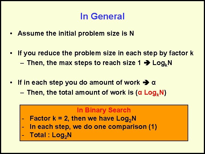
In General • Assume the initial problem size is N • If you reduce the problem size in each step by factor k – Then, the max steps to reach size 1 Logk. N • If in each step you do amount of work α – Then, the total amount of work is (α Logk. N) In Binary Search - Factor k = 2, then we have Log 2 N - In each step, we do one comparison (1) - Total : Log 2 N

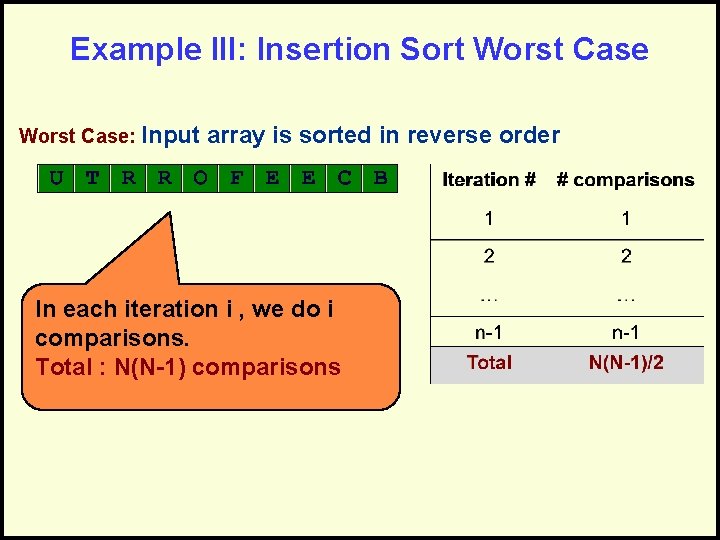
Example III: Insertion Sort Worst Case: Input array is sorted in reverse order In each iteration i , we do i comparisons. Total : N(N-1) comparisons

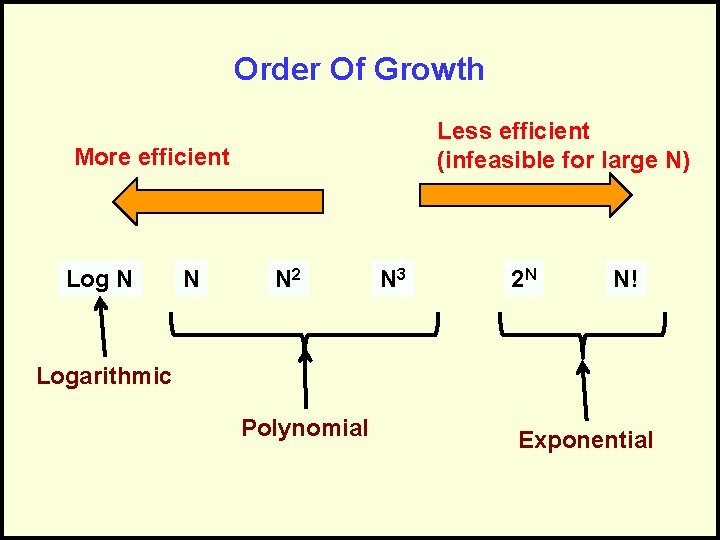
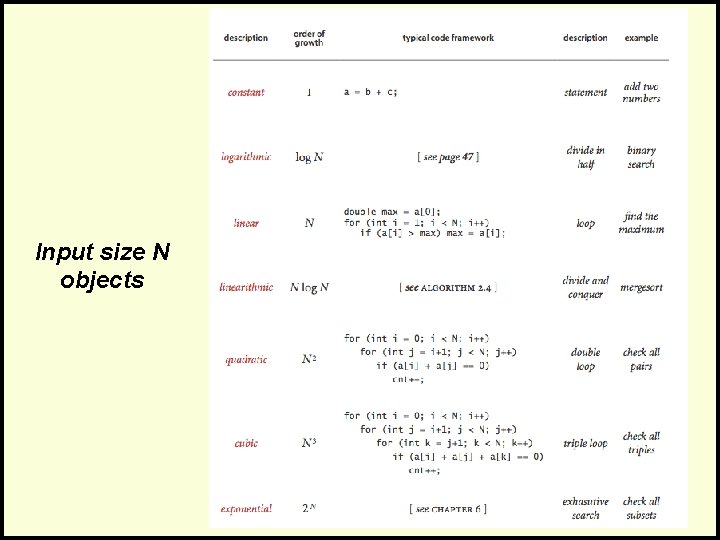
Order Of Growth Less efficient (infeasible for large N) More efficient Log N N N 2 N 3 2 N N! Logarithmic Polynomial Exponential

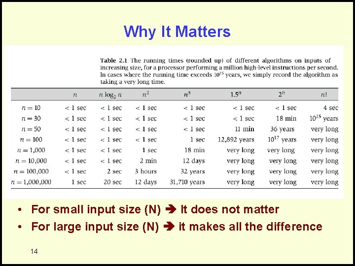
Why It Matters • For small input size (N) It does not matter • For large input size (N) it makes all the difference 14

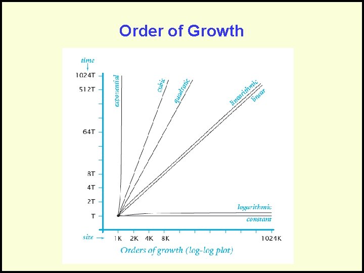
Order of Growth

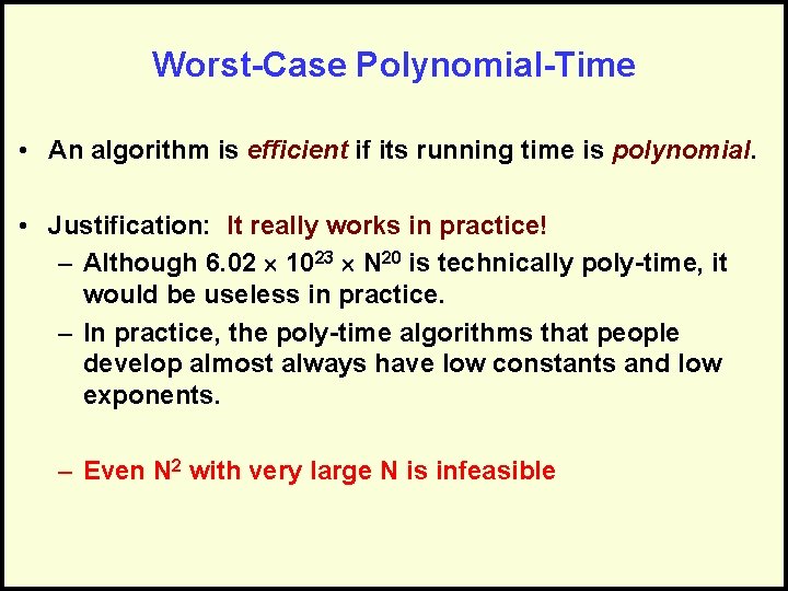
Worst-Case Polynomial-Time • An algorithm is efficient if its running time is polynomial. • Justification: It really works in practice! – Although 6. 02 1023 N 20 is technically poly-time, it would be useless in practice. – In practice, the poly-time algorithms that people develop almost always have low constants and low exponents. – Even N 2 with very large N is infeasible

Input size N objects

LB Introducing Big O • Will allow us to evaluate algorithms. • Has precise mathematical definition • Used in a sense to put algorithms into families

Why Use Big-O Notation • Used when we only know the asymptotic upper bound. • If you are not guaranteed certain input, then it is a valid upper bound that even the worstcase input will be below. • May often be determined by inspection of an algorithm. • Thus we don’t have to do a proof!

Size of Input • In analyzing rate of growth based upon size of input, we’ll use a variable – For each factor in the size, use a new variable – N is most common… Examples: – A linked list of N elements – A 2 D array of N x M elements – 2 Lists of size N and M elements – A Binary Search Tree of N elements

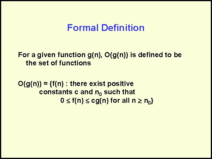
Formal Definition For a given function g(n), O(g(n)) is defined to be the set of functions O(g(n)) = {f(n) : there exist positive constants c and n 0 such that 0 f(n) cg(n) for all n n 0}

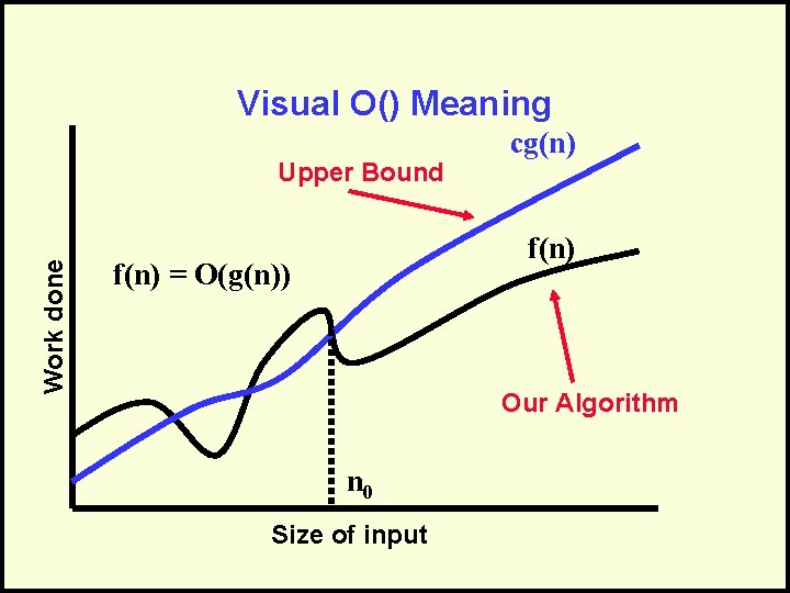
Visual O() Meaning Work done Upper Bound cg(n) f(n) = O(g(n)) Our Algorithm n 0 Size of input

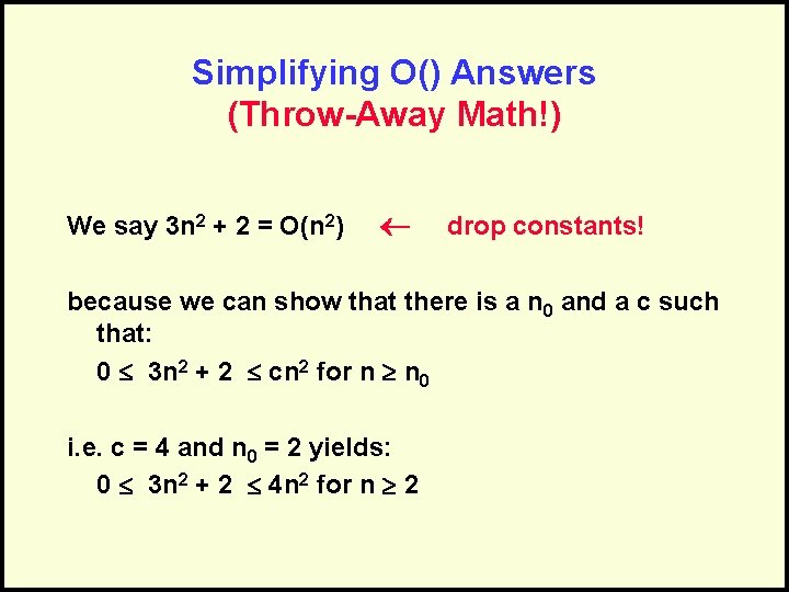
Simplifying O() Answers (Throw-Away Math!) We say 3 n 2 + 2 = O(n 2) drop constants! because we can show that there is a n 0 and a c such that: 0 3 n 2 + 2 cn 2 for n n 0 i. e. c = 4 and n 0 = 2 yields: 0 3 n 2 + 2 4 n 2 for n 2

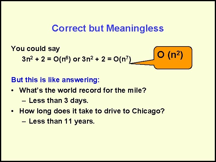
Correct but Meaningless You could say 3 n 2 + 2 = O(n 6) or 3 n 2 + 2 = O(n 7) O (n 2) But this is like answering: • What’s the world record for the mile? – Less than 3 days. • How long does it take to drive to Chicago? – Less than 11 years.

Comparing Algorithms • Now that we know the formal definition of O() notation (and what it means)… • If we can determine the O() of algorithms… • This establishes the worst they perform. • Thus now we can compare them and see which has the “better” performance.

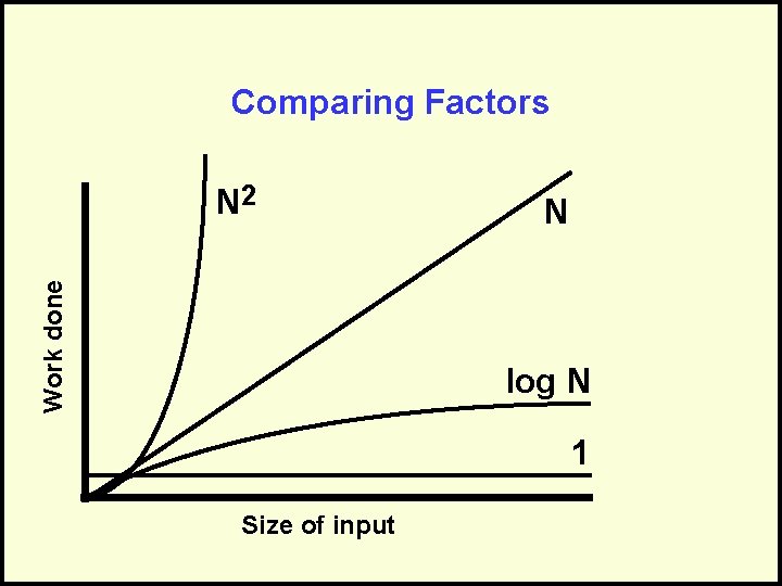
Comparing Factors Work done N 2 N log N 1 Size of input

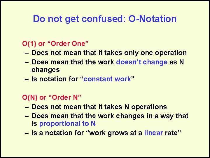
Do not get confused: O-Notation O(1) or “Order One” – Does not mean that it takes only one operation – Does mean that the work doesn’t change as N changes – Is notation for “constant work” O(N) or “Order N” – Does not mean that it takes N operations – Does mean that the work changes in a way that is proportional to N – Is a notation for “work grows at a linear rate”

Complex/Combined Factors • Algorithms typically consist of a sequence of logical steps/sections • We need a way to analyze these more complex algorithms… • It’s easy – analyze the sections and then combine them!

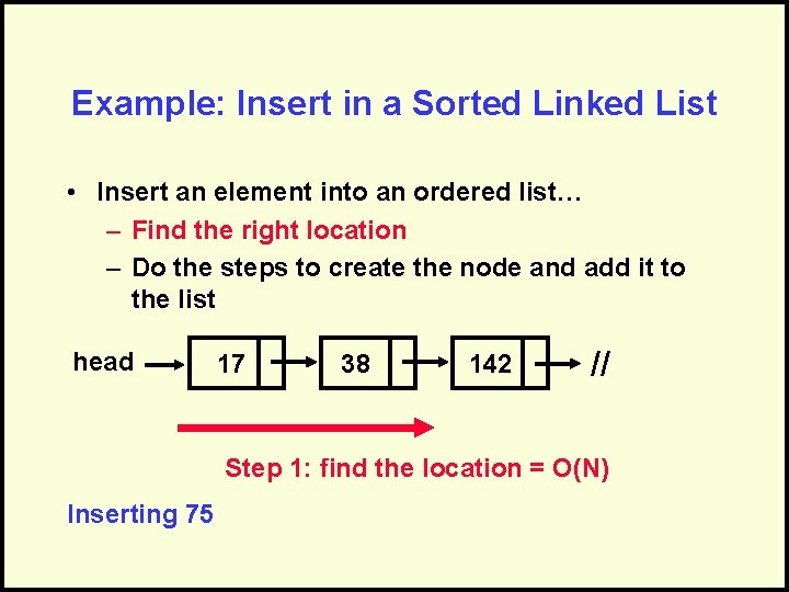
Example: Insert in a Sorted Linked List • Insert an element into an ordered list… – Find the right location – Do the steps to create the node and add it to the list head 17 38 142 // Step 1: find the location = O(N) Inserting 75

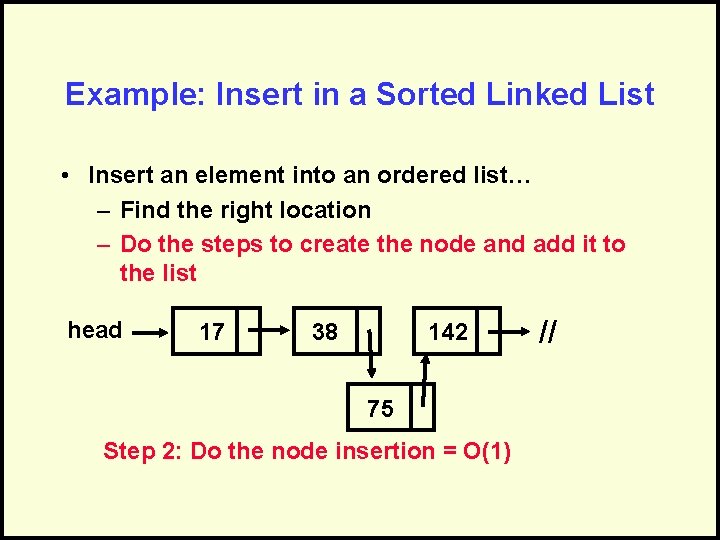
Example: Insert in a Sorted Linked List • Insert an element into an ordered list… – Find the right location – Do the steps to create the node and add it to the list head 17 38 142 75 Step 2: Do the node insertion = O(1) //

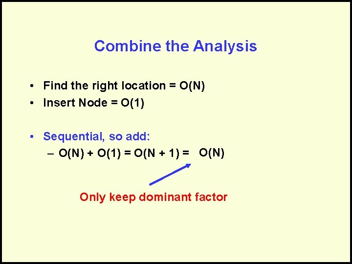
Combine the Analysis • Find the right location = O(N) • Insert Node = O(1) • Sequential, so add: – O(N) + O(1) = O(N + 1) = O(N) Only keep dominant factor

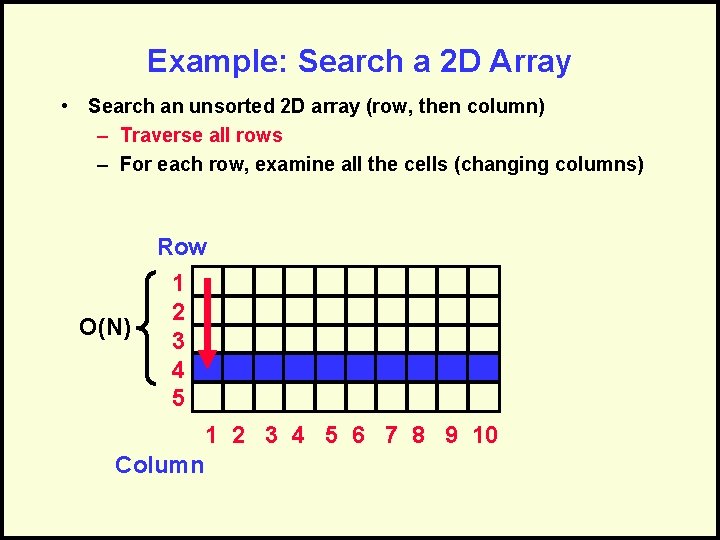
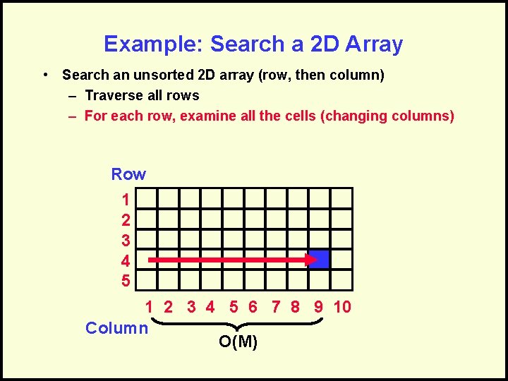
Example: Search a 2 D Array • Search an unsorted 2 D array (row, then column) – Traverse all rows – For each row, examine all the cells (changing columns) Row O(N) 1 2 3 4 5 6 7 8 9 10 Column

Example: Search a 2 D Array • Search an unsorted 2 D array (row, then column) – Traverse all rows – For each row, examine all the cells (changing columns) Row 1 2 3 4 5 6 7 8 9 10 Column O(M)

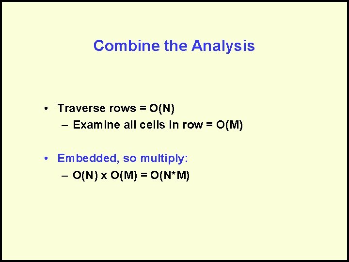
Combine the Analysis • Traverse rows = O(N) – Examine all cells in row = O(M) • Embedded, so multiply: – O(N) x O(M) = O(N*M)

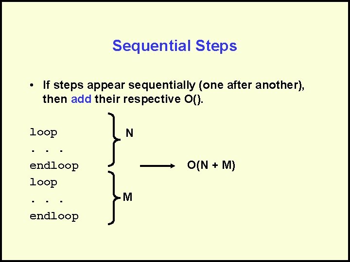
Sequential Steps • If steps appear sequentially (one after another), then add their respective O(). loop. . . endloop N O(N + M) M

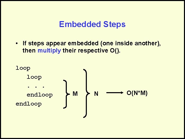
Embedded Steps • If steps appear embedded (one inside another), then multiply their respective O(). loop. . . endloop M N O(N*M)

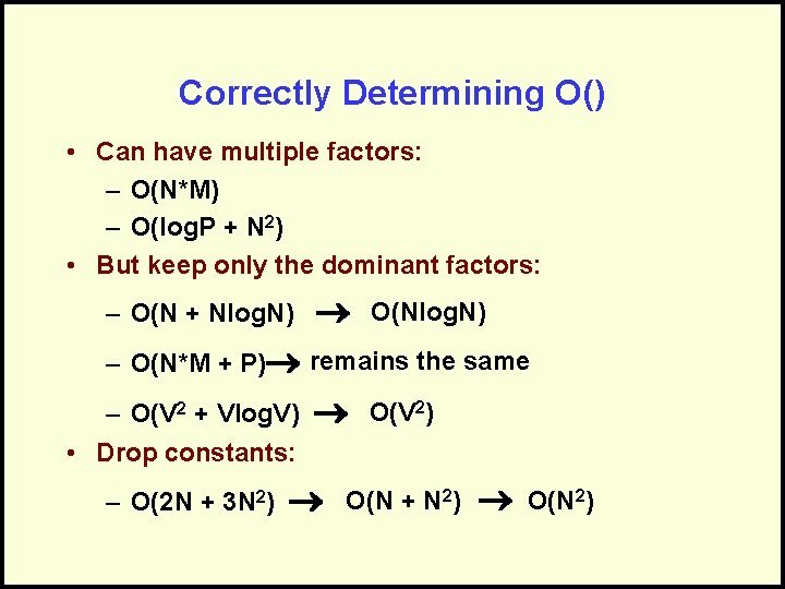
Correctly Determining O() • Can have multiple factors: – O(N*M) – O(log. P + N 2) • But keep only the dominant factors: – O(N + Nlog. N) O(Nlog. N) – O(N*M + P) remains the same – O(V 2 + Vlog. V) • Drop constants: – O(2 N + 3 N 2) O(V 2) O(N + N 2) O(N 2)

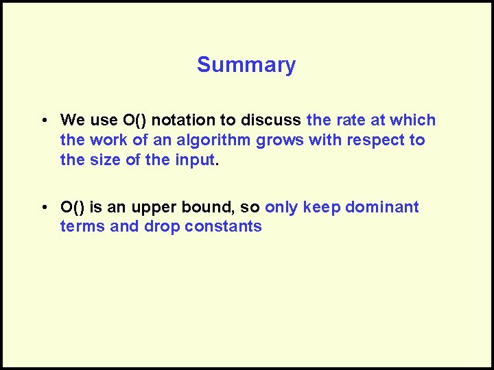
Summary • We use O() notation to discuss the rate at which the work of an algorithm grows with respect to the size of the input. • O() is an upper bound, so only keep dominant terms and drop constants