Algorithm Analysis Algorithm Analysis Algorithms stepbystep procedure for

Algorithm Analysis

Algorithm Analysis Algorithms: step-by-step procedure for performing some tasks in finite amount of time Analyse Algorithms ◦ Running time algorithms & data structure operators ◦ Space data structures

Example Searching for a name in a list of 10? If the size of the list is 100? 1000? If the list is sorted? Unsorted? Will there be any difference in the running time say of sorting 10 numbers or 100 numbers? Or say downloading an image of 100 KB or 2 MB or 30 MB?

Running Time Depends on ◦ Size of the input: as the size increases, usually the running time of algorithms or functions increase. ◦ Hardware environment: memory capacity, processor speed, hard disk space, clock speed etc. ◦ Software environment: operating system, programming language, compiler etc.

Algorithm Analysis Experimental General Studies Methodology Counting Primitive Operations Asymptotic Analysis

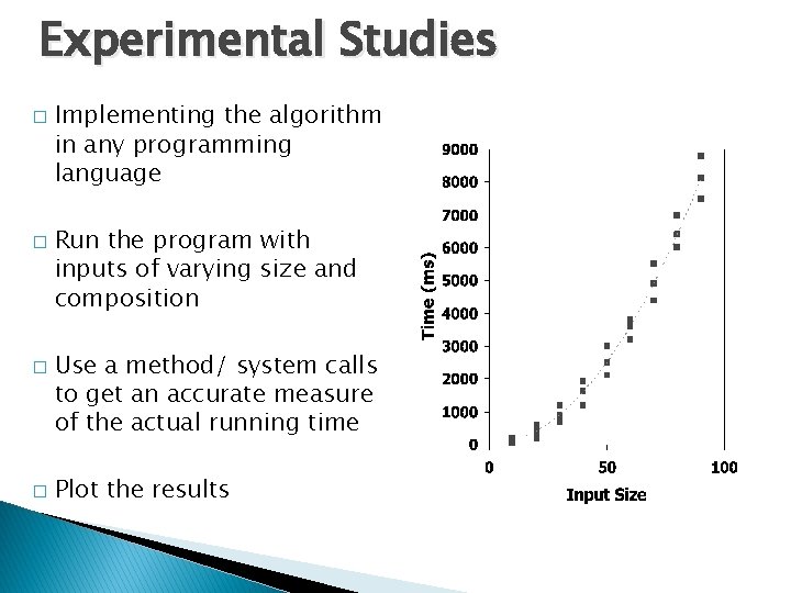
Experimental Studies � � Implementing the algorithm in any programming language Run the program with inputs of varying size and composition Use a method/ system calls to get an accurate measure of the actual running time Plot the results

Limitations of Experiments It is necessary to implement and execute the algorithm, which may be difficult and time consuming Results may not be indicative of the running time on other inputs not included in the experiment In order to compare two algorithms, the same hardware and software environments must be used

General Methodology/ Theoretical Analysis � Uses a high-level description of the algorithm instead of an implementation - pseudo code � Characterizes input size, n � Takes running time as a function of the into account all possible inputs � Allows us to evaluate the speed of an algorithm independent of the hardware/software environment

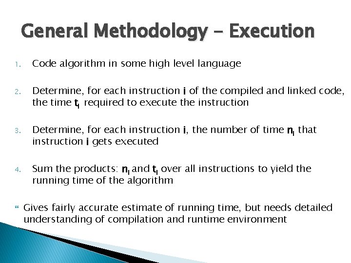
General Methodology - Execution 1. Code algorithm in some high level language 2. Determine, for each instruction i of the compiled and linked code, the time ti required to execute the instruction 3. Determine, for each instruction i, the number of time ni that instruction i gets executed 4. Sum the products: ni and ti over all instructions to yield the running time of the algorithm Gives fairly accurate estimate of running time, but needs detailed understanding of compilation and runtime environment

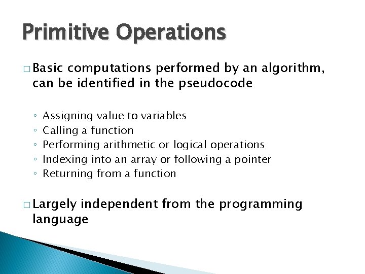
Primitive Operations � Basic computations performed by an algorithm, can be identified in the pseudocode ◦ ◦ ◦ Assigning value to variables Calling a function Performing arithmetic or logical operations Indexing into an array or following a pointer Returning from a function � Largely independent from the programming language

Primitive Operations This approach of estimating the running time of an algorithm is based on the assumption that given a h/w and a s/w environment, the execution time of each low level instruction corresponding to each primitive operation, will be constant So if we count the maximum number of primitive operations executed in an algorithm, we can get a high level estimate of the running time of the algorithm

Example // Assume A [] to be an array of integers of size n curr. Large = 0 for (i=0; i<n; i++) { if A [curr. Large] < A [i] curr. Large = i } return currlarge What would be the best case and the worst case for this code?

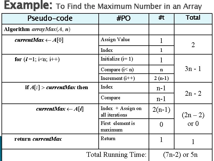
Example: To Find the Maximum Number in an Array Pseudo-code #PO #t Assign Value 1 Index 1 Initialize (i= 1) 1 Compare (i< n) n Increment (i++) 2 (n-1) Total Algorithm array. Max(A, n) current. Max A[0] for (i =1; i<n; i++) if A[i] current. Max then Index Compare current. Max A[i] return current. Max Index + Assign on all iterations 2 3 n - 1 n-1 2(n-1) 2 n - 2 First element is maximum 0 (2 n – 2) or 0 Return 1 1 Total Running Time: (7 n-2) or 5 n

Example. . Best Case: when A[0] is the largest element and the variable current. Max is never reassigned. The number of PO executed is least at 5 n. Worst Case: when array elements are sorted in increasing order and the variable current. Max is reassigned on every iteration. The number of PO executed is 7 n - 2

Worse Case Analysis Running times are mostly characterised in terms of their worst case – the maximum number of primitive operations executed by the algorithm, taken over all inputs of size particular size ◦ Analysis easier than average case ◦ May actually lead to better algorithms

Point to Ponder Average case analysis expresses the running time of algorithms as an average taken over all possible inputs. What are the possible drawbacks of this approach as compared to the worse case analysis? Why should one restrain from doing the best case analysis of any algorithms?

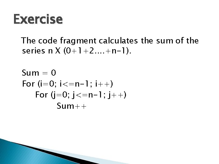
Exercise The code fragment calculates the sum of the series n X (0+1+2. . +n-1). Sum = 0 For (i=0; i<=n-1; i++) For (j=0; j<=n-1; j++) Sum++

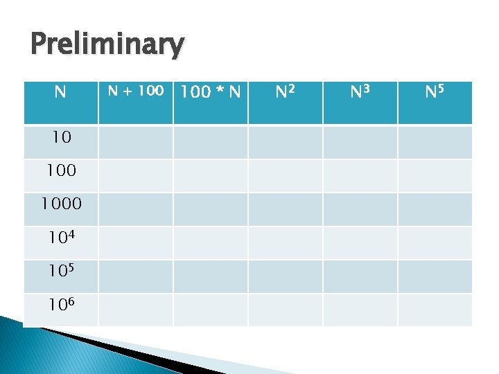
Preliminary N 10 1000 104 105 106 N + 100 * N N 2 N 3 N 5

Growth Rate Growth rate for an algorithm is the rate at which the running time of the algorithm (or the cost) grows as the size of its input grows.

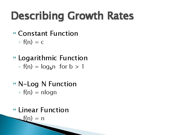
Describing Growth Rates Constant Function ◦ f(n) = c Logarithmic Function ◦ f(n) = logbn for b > 1 N-Log N Function ◦ f(n) = nlogn Linear Function ◦ f(n) = n

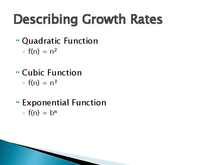
Describing Growth Rates Quadratic Function ◦ f(n) = n 2 Cubic Function ◦ f(n) = n 3 Exponential Function ◦ f(n) = bn

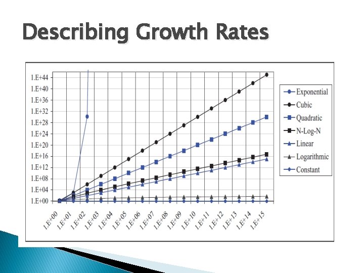
Describing Growth Rates

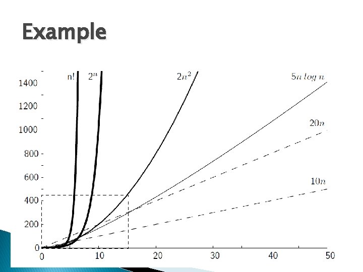
Example Graph and figure/table

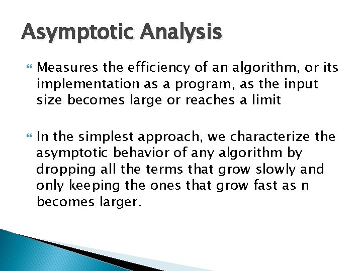
Asymptotic Analysis Measures the efficiency of an algorithm, or its implementation as a program, as the input size becomes large or reaches a limit In the simplest approach, we characterize the asymptotic behavior of any algorithm by dropping all the terms that grow slowly and only keeping the ones that grow fast as n becomes larger.

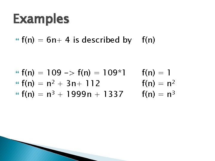
Examples f(n) = 6 n+ 4 is described by f(n) = 109 -> f(n) = 109*1 f(n) = n 2 + 3 n+ 112 f(n) = n 3 + 1999 n + 1337 f(n) = 1 f(n) = n 2 f(n) = n 3

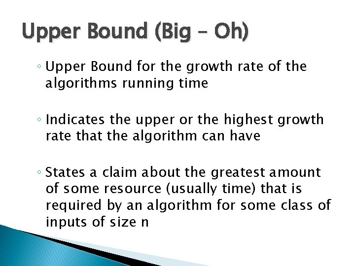
Upper Bound (Big – Oh) ◦ Upper Bound for the growth rate of the algorithms running time ◦ Indicates the upper or the highest growth rate that the algorithm can have ◦ States a claim about the greatest amount of some resource (usually time) that is required by an algorithm for some class of inputs of size n

Lower Bound (big Ω) Describes the least amount of a resource that an algorithm needs for some particular class of inputs – the worst, average, or best case input of size n The notations are usually used when the asymptotic behavior of the algorithm cannot be expressed by simple algebraic operations or thru intuitive notions

Determining Complexity Simple assignment statement ◦ Marks =100 ◦ A[i] = 0 ◦ f(n) = c or f(n) = 1 Any program that doesn't have any loops will have f( n ) = 1, since the number of instructions it needs is just a constant (unless it uses recursion).

Determining Complexity Simple programs can be analyzed by counting the nested loops of the program. ◦ A single loop over n items yields f( n ) = n ◦ A loop within a loop yields f( n ) = n 2. ◦ A loop within a loop yields f( n ) = n 3. ◦ Given a series of for loops that are sequential, the slowest of them determines the asymptotic behaviour of the program.

Determining Complexity Two nested loops followed by a single loop is asymptotically the same as the nested loops alone because the nested loops dominate the simple loop If we have a program that calls a function within a loop and we know the number of instructions the called function performs, it's easy to determine the number of instructions of the whole program.

References http: //discrete. gr/complexity/ Goodrich et. al. / Chapter 4 Shaffer et. Al. / Chapter 3