Algorithm Analysis 1 Introduction What is an algorithm

Algorithm Analysis 1

Introduction What is an algorithm? An algorithm is a sequence of unambiguous instructions for solving a problem 2 • Can be represented various forms • Unambiguity/clearness • Effectiveness • Finiteness/termination • Correctness

Basic Issues Related to Algorithms How to design algorithms How to express algorithms Proving correctness Efficiency (or complexity) analysis Theoretical analysis Empirical analysis Optimality

Analysis of Algorithms How good is the algorithm? Correctness Time efficiency Space efficiency Does there exist a better algorithm? Lower bounds Optimality

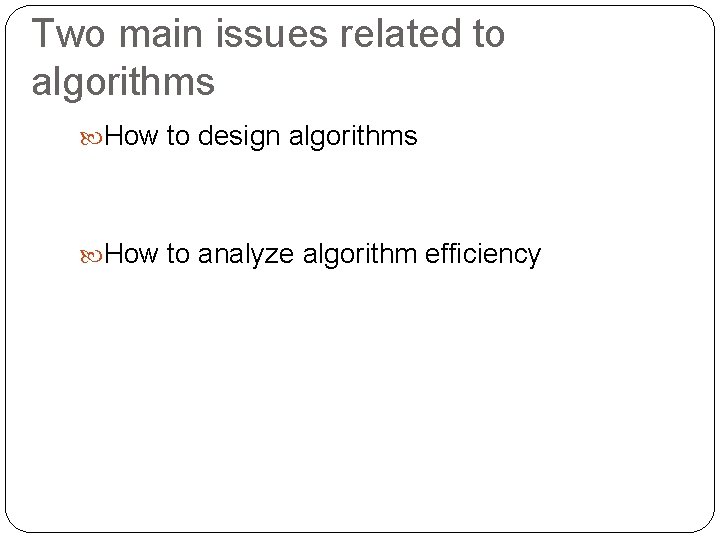
Two main issues related to algorithms How to design algorithms How to analyze algorithm efficiency

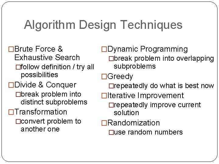
Algorithm Design Techniques �Brute Force & Exhaustive Search �follow definition / try all possibilities �Divide & Conquer �break problem into distinct subproblems �Transformation �convert problem to another one 6 �Dynamic Programming �break problem into overlapping subproblems �Greedy �repeatedly do what is best now �Iterative Improvement �repeatedly improve current solution �Randomization �use random numbers

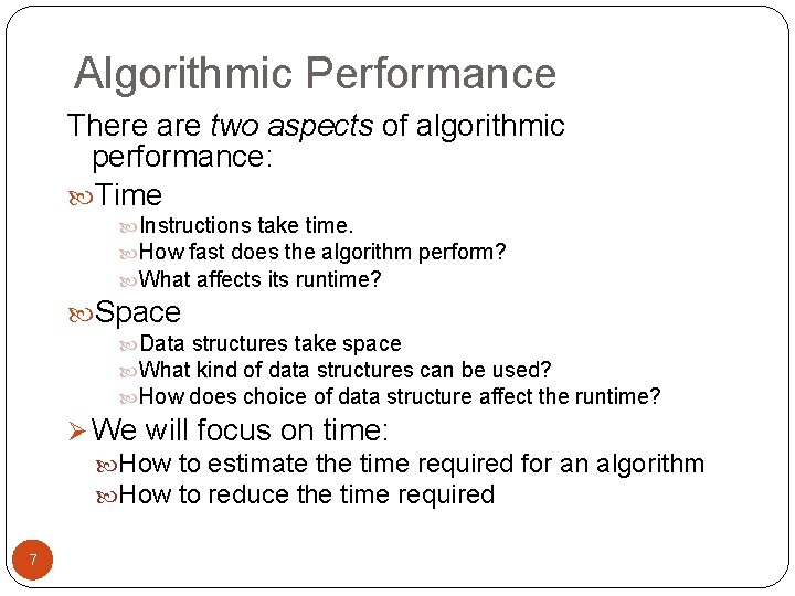
Algorithmic Performance There are two aspects of algorithmic performance: Time Instructions take time. How fast does the algorithm perform? What affects its runtime? Space Data structures take space What kind of data structures can be used? How does choice of data structure affect the runtime? Ø We will focus on time: How to estimate the time required for an algorithm How to reduce the time required 7

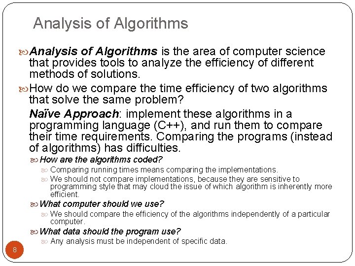
Analysis of Algorithms is the area of computer science that provides tools to analyze the efficiency of different methods of solutions. How do we compare the time efficiency of two algorithms that solve the same problem? Naïve Approach: implement these algorithms in a programming language (C++), and run them to compare their time requirements. Comparing the programs (instead of algorithms) has difficulties. How are the algorithms coded? Comparing running times means comparing the implementations. We should not compare implementations, because they are sensitive to programming style that may cloud the issue of which algorithm is inherently more efficient. What computer should we use? We should compare the efficiency of the algorithms independently of a particular computer. What data should the program use? Any analysis must be independent of specific data. 8

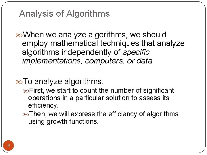
Analysis of Algorithms When we analyze algorithms, we should employ mathematical techniques that analyze algorithms independently of specific implementations, computers, or data. To analyze algorithms: First, we start to count the number of significant operations in a particular solution to assess its efficiency. Then, we will express the efficiency of algorithms using growth functions. 9

Important problem types sorting searching string processing graph problems combinatorial problems geometric problems numerical problems

Asymptotic Performance 11

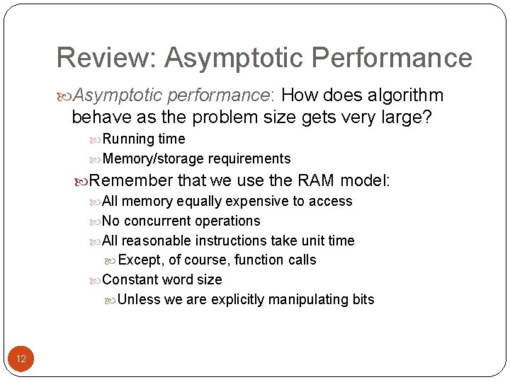
Review: Asymptotic Performance Asymptotic performance: How does algorithm behave as the problem size gets very large? Running time Memory/storage requirements Remember that we use the RAM model: All memory equally expensive to access No concurrent operations All reasonable instructions take unit time Except, of course, function calls Constant word size Unless we are explicitly manipulating bits 12

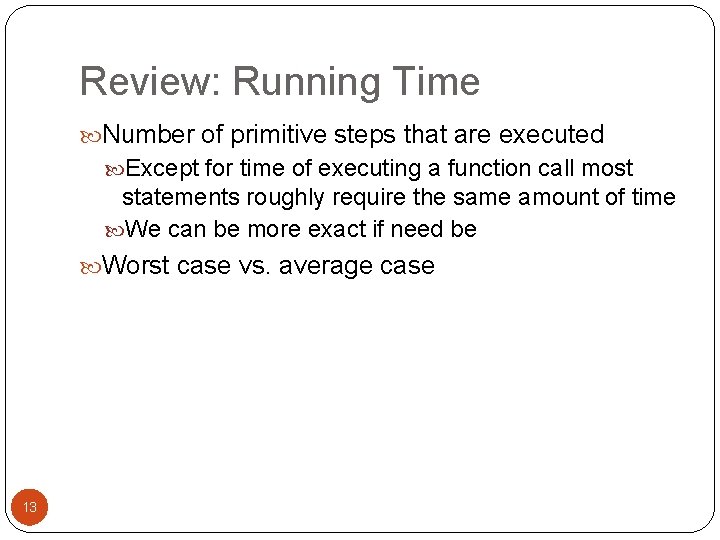
Review: Running Time Number of primitive steps that are executed Except for time of executing a function call most statements roughly require the same amount of time We can be more exact if need be Worst case vs. average case 13

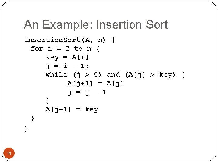
An Example: Insertion Sort Insertion. Sort(A, n) { for i = 2 to n { key = A[i] j = i - 1; while (j > 0) and (A[j] > key) { A[j+1] = A[j] j = j - 1 } A[j+1] = key } } 14

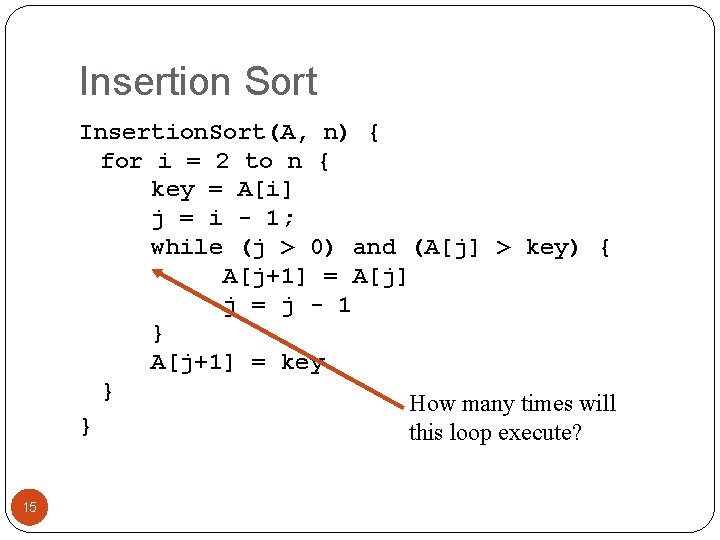
Insertion Sort Insertion. Sort(A, n) { for i = 2 to n { key = A[i] j = i - 1; while (j > 0) and (A[j] > key) { A[j+1] = A[j] j = j - 1 } A[j+1] = key } How many times will } this loop execute? 15

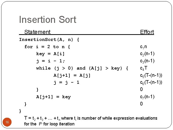
Insertion Sort Statement 16 Effort Insertion. Sort(A, n) { for i = 2 to n { c 1 n key = A[i] c 2(n-1) j = i - 1; c 3(n-1) while (j > 0) and (A[j] > key) { c 4 T A[j+1] = A[j] c 5(T-(n-1)) j = j - 1 c 6(T-(n-1)) } 0 A[j+1] = key c 7(n-1) } 0 } T = t 2 + t 3 + … + tn where ti is number of while expression evaluations for the ith for loop iteration

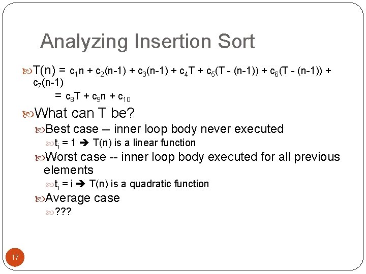
Analyzing Insertion Sort T(n) = c 1 n + c 2(n-1) + c 3(n-1) + c 4 T + c 5(T - (n-1)) + c 6(T - (n-1)) + c 7(n-1) = c 8 T + c 9 n + c 10 What can T be? Best case -- inner loop body never executed ti = 1 T(n) is a linear function Worst case -- inner loop body executed for all previous elements ti = i T(n) is a quadratic function Average case ? ? ? 17

Analysis Simplifications Ignore actual and abstract statement costs Order of growth is the interesting measure: Highest-order term is what counts Remember, we are doing asymptotic analysis As the input size grows larger it is the high order term that dominates 18

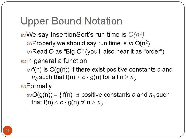
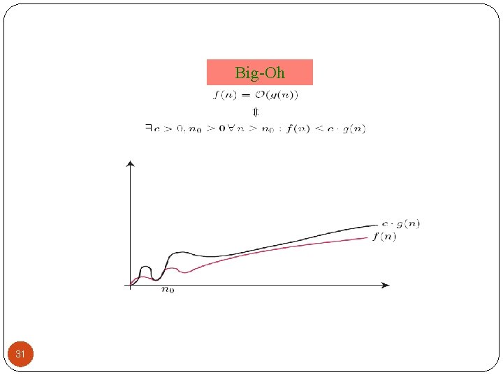
Upper Bound Notation We say Insertion. Sort’s run time is O(n 2) Properly we should say run time is in O(n 2) Read O as “Big-O” (you’ll also hear it as “order”) In general a function f(n) is O(g(n)) if there exist positive constants c and n 0 such that f(n) c g(n) for all n n 0 Formally O(g(n)) = { f(n): positive constants c and n 0 such that f(n) c g(n) n n 0 19

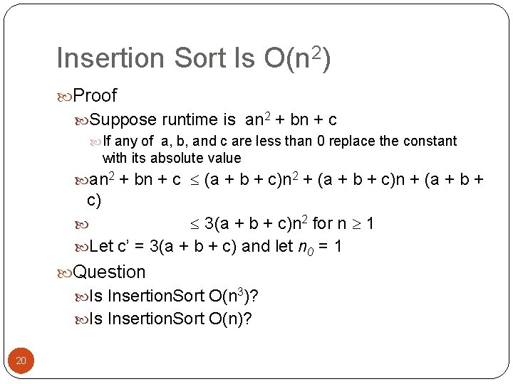
Insertion Sort Is O(n 2) Proof Suppose runtime is an 2 + bn + c If any of a, b, and c are less than 0 replace the constant with its absolute value an 2 + bn + c (a + b + c)n 2 + (a + b + c)n + (a + b + c) 3(a + b + c)n 2 for n 1 Let c’ = 3(a + b + c) and let n 0 = 1 Question Is Insertion. Sort O(n 3)? Is Insertion. Sort O(n)? 20

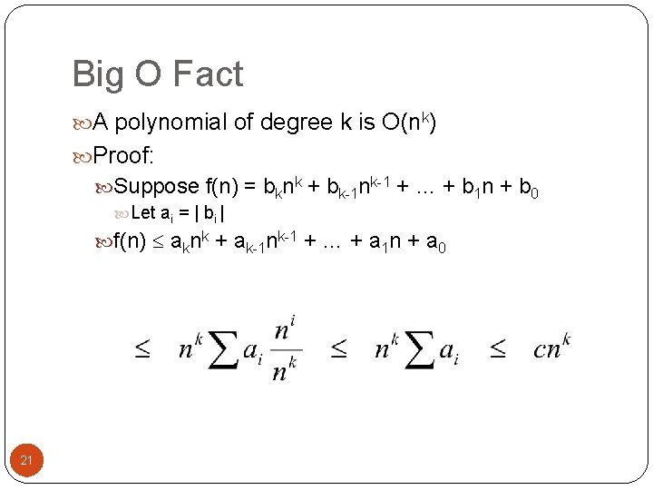
Big O Fact A polynomial of degree k is O(nk) Proof: Suppose f(n) = bknk + bk-1 nk-1 + … + b 1 n + b 0 Let ai = | bi | f(n) aknk + ak-1 nk-1 + … + a 1 n + a 0 21

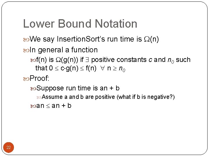
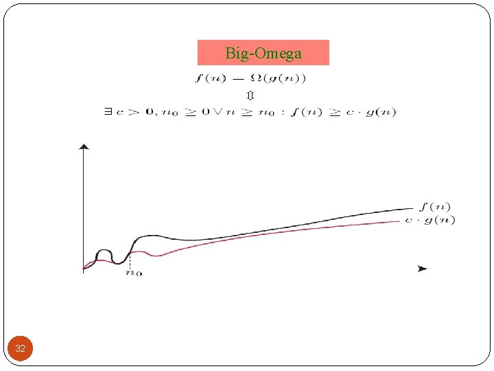
Lower Bound Notation We say Insertion. Sort’s run time is (n) In general a function f(n) is (g(n)) if positive constants c and n 0 such that 0 c g(n) f(n) n n 0 Proof: Suppose run time is an + b Assume a and b are positive (what if b is negative? ) an + b 22

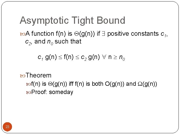
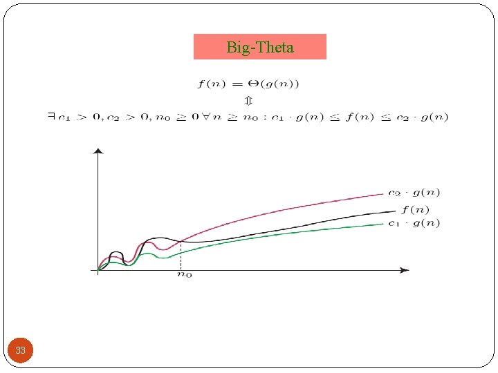
Asymptotic Tight Bound A function f(n) is (g(n)) if positive constants c 1, c 2, and n 0 such that c 1 g(n) f(n) c 2 g(n) n n 0 Theorem f(n) is (g(n)) iff f(n) is both O(g(n)) and (g(n)) Proof: someday 23

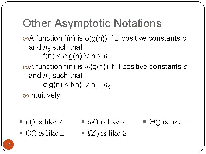
Other Asymptotic Notations A function f(n) is o(g(n)) if positive constants c and n 0 such that f(n) < c g(n) n n 0 A function f(n) is (g(n)) if positive constants c and n 0 such that c g(n) < f(n) n n 0 Intuitively, § o() is like < § O() is like 24 § () is like > § () is like =

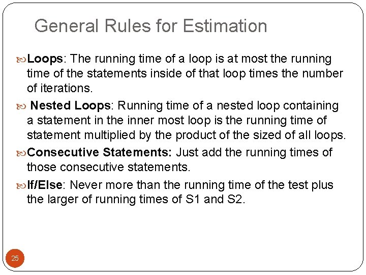
General Rules for Estimation Loops: The running time of a loop is at most the running time of the statements inside of that loop times the number of iterations. Nested Loops: Running time of a nested loop containing a statement in the inner most loop is the running time of statement multiplied by the product of the sized of all loops. Consecutive Statements: Just add the running times of those consecutive statements. If/Else: Never more than the running time of the test plus the larger of running times of S 1 and S 2. 25

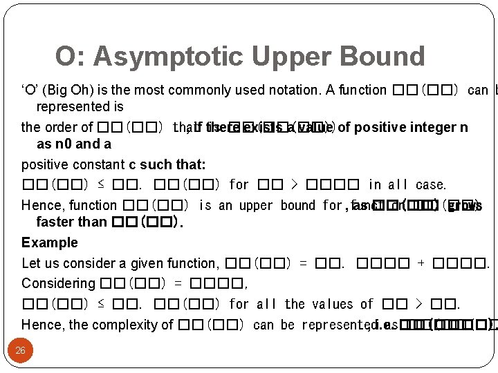
O: Asymptotic Upper Bound ‘O’ (Big Oh) is the most commonly used notation. A function ��(��) can b represented is the order of ��(��) that , if there is ��(��(��)) exists a value of positive integer n as n 0 and a positive constant c such that: ��(��) ≤ ��. ��(��) for �� > ���� in all case. Hence, function ��(��) is an upper bound for , function as ��(��) grows faster than ��(��). Example Let us consider a given function, ��(��) = ��. ���� + ����. Considering ��(��) = ����, ��(��) ≤ ��. ��(��) for all the values of �� > ��. Hence, the complexity of ��(��) can be represented , i. e. as��(����). ��(��(�� 26

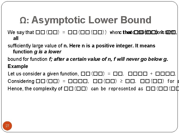
Ω: Asymptotic Lower Bound We say that ��(��) = ��(��(��)) whenc there that ��(��) exists constant ≥ ��. all sufficiently large value of n. Here n is a positive integer. It means function g is a lower bound for function f; after a certain value of n, f will never go below g. Example Let us consider a given function, ��(��) = ��. ���� + ����. Considering ��(��) = ����, ��(��) ≥ ��. ��(��) for a Hence, the complexity of ��(��) can be represented as ��(��(�� 27

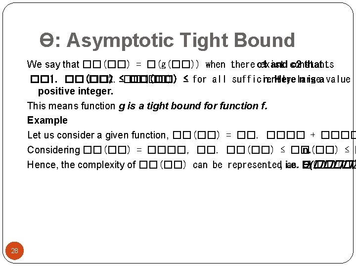
Ɵ: Asymptotic Tight Bound We say that ��(��) = �(g(��)) when there c 1 exist and constants c 2 that �� 1. ��(��) �� 2. ≤��(��) ≤ for all sufficiently n. Herelarge n is a value o positive integer. This means function g is a tight bound for function f. Example Let us consider a given function, ��(��) = ��. ���� + ���� Considering ��(��) = ����, ��. ��(��) ≤ ��(��) n. ≤ � Hence, the complexity of ��(��) can be represented, i. e. as �(��(�� Ɵ(����) 28

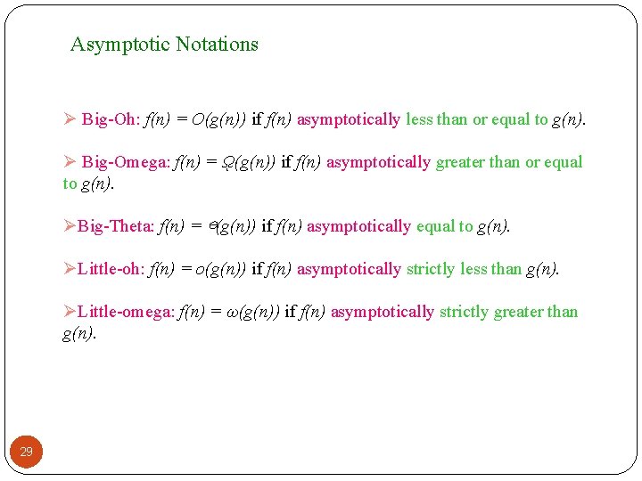
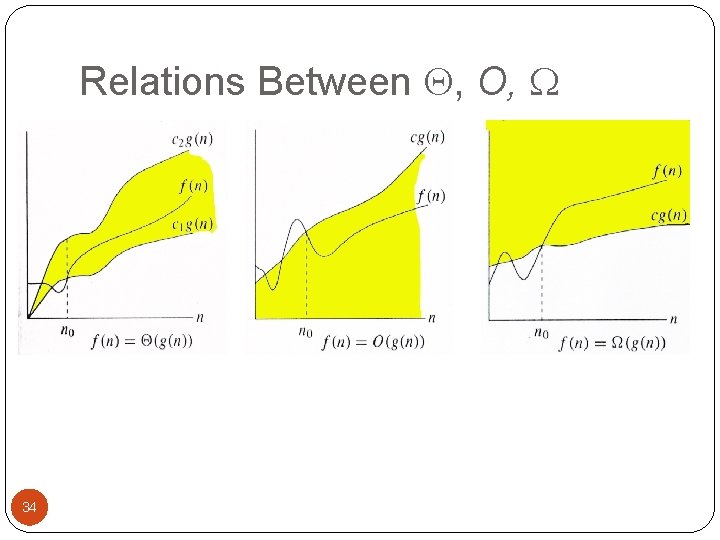
Asymptotic Notations Ø Big-Oh: f(n) = O(g(n)) if f(n) asymptotically less than or equal to g(n). Ø Big-Omega: f(n) = ῼ(g(n)) if f(n) asymptotically greater than or equal to g(n). ØBig-Theta: f(n) = ⊖(g(n)) if f(n) asymptotically equal to g(n). ØLittle-oh: f(n) = o(g(n)) if f(n) asymptotically strictly less than g(n). ØLittle-omega: f(n) = ω(g(n)) if f(n) asymptotically strictly greater than g(n). 29

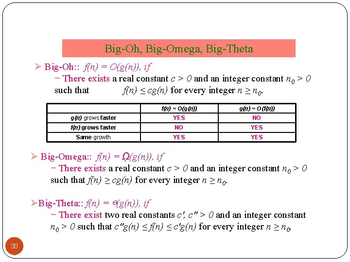
Big-Oh, Big-Omega, Big-Theta Ø Big-Oh: : f(n) = O(g(n)), if − There exists a real constant c > 0 and an integer constant n 0 > 0 such that f(n) ≤ cg(n) for every integer n ≥ n 0. f(n) = O(g(n)) g(n) = O(f(n)) g(n) grows faster YES NO f(n) grows faster NO YES Same growth YES Ø Big-Omega: : f(n) = ῼ(g(n)), if − There exists a real constant c > 0 and an integer constant n 0 > 0 such that f(n) ≥ cg(n) for every integer n ≥ n 0. ØBig-Theta: : f(n) = ⊖(g(n)), if − There exist two real constants c′, c′′ > 0 and an integer constant n 0 > 0 such that c′′g(n) ≤ f(n) ≤ c′g(n) for every integer n ≥ n 0. 30

Big-Oh 31

Big-Omega 32

Big-Theta 33

Relations Between , O, 34

Algorithm Growth Rates � We measure an algorithm’s time requirement as a function of the problem size. �Problem size depends on the application: e. g. number of elements in a list for a sorting algorithm, the number disks for towers of hanoi. � So, for instance, we say that (if the problem size is n) �Algorithm A requires 5*n 2 time units to solve a problem of size n. �Algorithm B requires 7*n time units to solve a problem of size n. � The most important thing to learn is how quickly the algorithm’s time requirement grows as a function of the problem size. �Algorithm A requires time proportional to n 2. �Algorithm B requires time proportional to n. � An algorithm’s proportional time requirement is known 35 as growth rate. � We can compare the efficiency of two algorithms by comparing their growth rates.

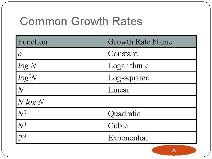
Common Growth Rates Function c log N log 2 N N N log N N 2 N 3 2 N Growth Rate Name Constant Logarithmic Log-squared Linear Quadratic Cubic Exponential 36

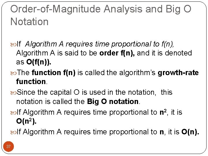
Order-of-Magnitude Analysis and Big O Notation If Algorithm A requires time proportional to f(n), Algorithm A is said to be order f(n), and it is denoted as O(f(n)). The function f(n) is called the algorithm’s growth-rate function. Since the capital O is used in the notation, this notation is called the Big O notation. If Algorithm A requires time proportional to n 2, it is O(n 2). If Algorithm A requires time proportional to n, it is O(n). 37

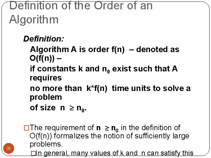
Definition of the Order of an Algorithm Definition: Algorithm A is order f(n) – denoted as O(f(n)) – if constants k and n 0 exist such that A requires no more than k*f(n) time units to solve a problem of size n n 0. �The requirement of n n 0 in the definition of 38 O(f(n)) formalizes the notion of sufficiently large problems. �In general, many values of k and n can satisfy this

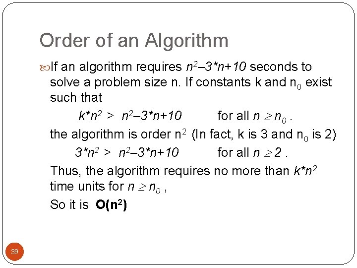
Order of an Algorithm If an algorithm requires n 2– 3*n+10 seconds to solve a problem size n. If constants k and n 0 exist such that k*n 2 > n 2– 3*n+10 for all n n 0. the algorithm is order n 2 (In fact, k is 3 and n 0 is 2) 3*n 2 > n 2– 3*n+10 for all n 2. Thus, the algorithm requires no more than k*n 2 time units for n n 0 , So it is O(n 2) 39

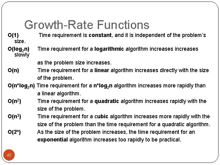
Growth-Rate Functions O(1) size. O(log 2 n) slowly Time requirement is constant, and it is independent of the problem’s Time requirement for a logarithmic algorithm increases as the problem size increases. O(n) Time requirement for a linear algorithm increases directly with the size of the problem. O(n*log 2 n) Time requirement for a n*log 2 n algorithm increases more rapidly than a linear algorithm. O(n 2) Time requirement for a quadratic algorithm increases rapidly with the size of the problem. O(n 3) Time requirement for a cubic algorithm increases more rapidly with the size of the problem than the time requirement for a quadratic algorithm. O(2 n) As the size of the problem increases, the time requirement for an exponential algorithm increases too rapidly to be practical. 40

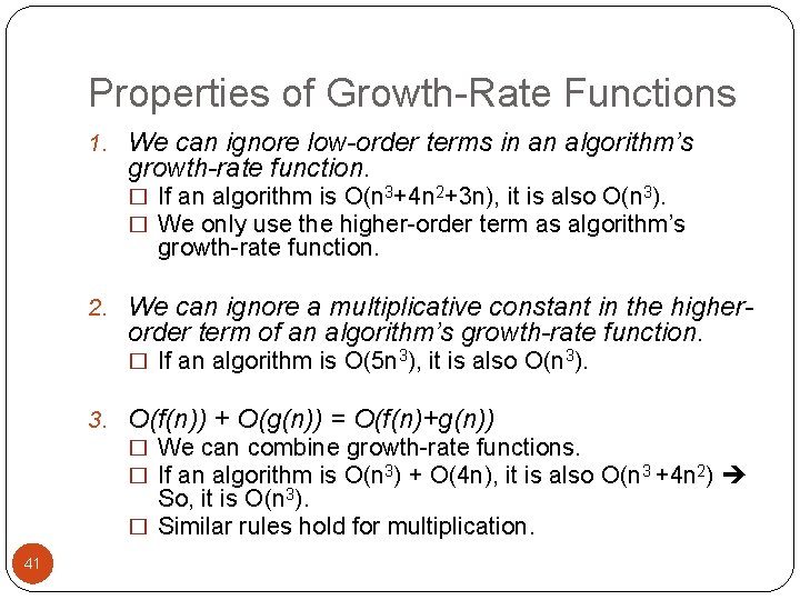
Properties of Growth-Rate Functions 1. We can ignore low-order terms in an algorithm’s growth-rate function. � If an algorithm is O(n 3+4 n 2+3 n), it is also O(n 3). � We only use the higher-order term as algorithm’s growth-rate function. 2. We can ignore a multiplicative constant in the higher- order term of an algorithm’s growth-rate function. � If an algorithm is O(5 n 3), it is also O(n 3). 3. O(f(n)) + O(g(n)) = O(f(n)+g(n)) � We can combine growth-rate functions. � If an algorithm is O(n 3) + O(4 n), it is also O(n 3 +4 n 2) So, it is O(n 3). � Similar rules hold for multiplication. 41

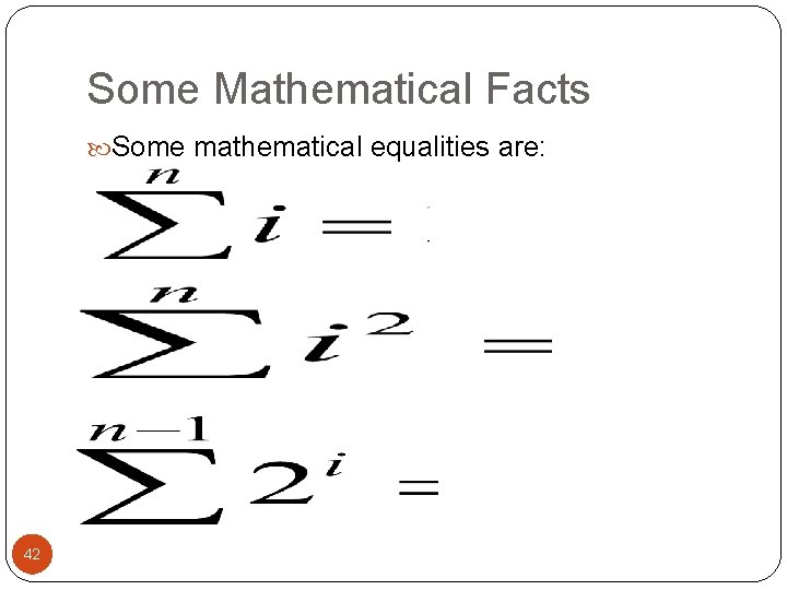
Some Mathematical Facts Some mathematical equalities are: 42

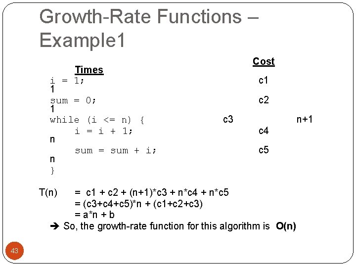
Growth-Rate Functions – Example 1 Times i = 1; 1 sum = 0; 1 while (i <= n) { i = i + 1; n sum = sum + i; n } T(n) Cost c 1 c 2 c 3 n+1 c 4 c 5 = c 1 + c 2 + (n+1)*c 3 + n*c 4 + n*c 5 = (c 3+c 4+c 5)*n + (c 1+c 2+c 3) = a*n + b So, the growth-rate function for this algorithm is O(n) 43

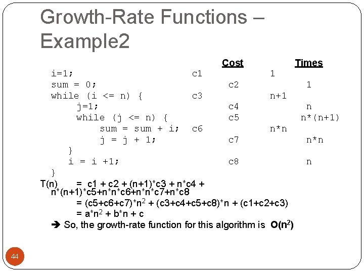
Growth-Rate Functions – Example 2 Cost Times i=1; c 1 1 sum = 0; c 2 1 while (i <= n) { c 3 n+1 j=1; c 4 n while (j <= n) { c 5 n*(n+1) sum = sum + i; c 6 n*n j = j + 1; c 7 n*n } i = i +1; c 8 n } T(n) = c 1 + c 2 + (n+1)*c 3 + n*c 4 + n*(n+1)*c 5+n*n*c 6+n*n*c 7+n*c 8 = (c 5+c 6+c 7)*n 2 + (c 3+c 4+c 5+c 8)*n + (c 1+c 2+c 3) = a*n 2 + b*n + c So, the growth-rate function for this algorithm is O(n 2) 44

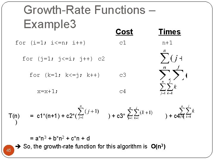
Growth-Rate Functions – Example 3 Cost for (i=1; i<=n; i++) c 1 Times n+1 for (j=1; j<=i; j++) c 2 for (k=1; k<=j; k++) x=x+1; T(n) ) 45 = c 1*(n+1) + c 2*( c 3 c 4 ) + c 3* ( ) + c 4*( = a*n 3 + b*n 2 + c*n + d So, the growth-rate function for this algorithm is O(n 3)

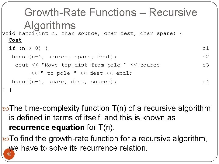
Growth-Rate Functions – Recursive Algorithms void hanoi(int n, char source, char dest, char spare) { Cost if (n > 0) { hanoi(n-1, source, spare, dest); cout << "Move top disk from pole " << source c 1 c 2 c 3 << " to pole " << dest << endl; hanoi(n-1, spare, dest, source); c 4 } } The time-complexity function T(n) of a recursive algorithm is defined in terms of itself, and this is known as recurrence equation for T(n). To find the growth-rate function for a recursive algorithm, we have to solve its recurrence relation. 46

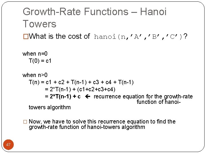
Growth-Rate Functions – Hanoi Towers �What is the cost of hanoi(n, ’A’, ’B’, ’C’)? when n=0 T(0) = c 1 when n>0 T(n) = c 1 + c 2 + T(n-1) + c 3 + c 4 + T(n-1) = 2*T(n-1) + (c 1+c 2+c 3+c 4) = 2*T(n-1) + c recurrence equation for the growth-rate function of hanoitowers algorithm � Now, we have to solve this recurrence equation to find the growth-rate function of hanoi-towers algorithm 47

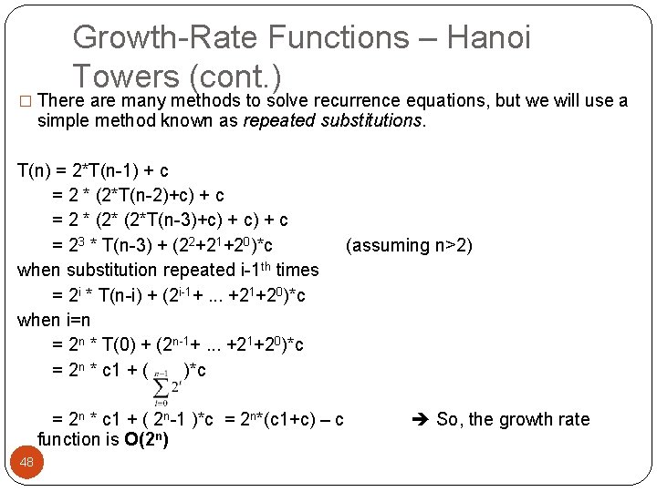
Growth-Rate Functions – Hanoi Towers (cont. ) � There are many methods to solve recurrence equations, but we will use a simple method known as repeated substitutions. T(n) = 2*T(n-1) + c = 2 * (2*T(n-2)+c) + c = 2 * (2*T(n-3)+c) + c = 23 * T(n-3) + (22+21+20)*c when substitution repeated i-1 th times = 2 i * T(n-i) + (2 i-1+. . . +21+20)*c when i=n = 2 n * T(0) + (2 n-1+. . . +21+20)*c = 2 n * c 1 + ( 2 n-1 )*c = 2 n*(c 1+c) – c function is O(2 n) 48 (assuming n>2) So, the growth rate

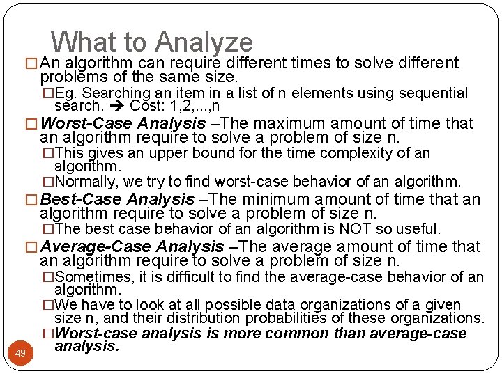
What to Analyze � An algorithm can require different times to solve different problems of the same size. �Eg. Searching an item in a list of n elements using sequential search. Cost: 1, 2, . . . , n � Worst-Case Analysis –The maximum amount of time that an algorithm require to solve a problem of size n. �This gives an upper bound for the time complexity of an algorithm. �Normally, we try to find worst-case behavior of an algorithm. � Best-Case Analysis –The minimum amount of time that an algorithm require to solve a problem of size n. �The best case behavior of an algorithm is NOT so useful. � Average-Case Analysis –The average amount of time that an algorithm require to solve a problem of size n. �Sometimes, it is difficult to find the average-case behavior of an 49 algorithm. �We have to look at all possible data organizations of a given size n, and their distribution probabilities of these organizations. �Worst-case analysis is more common than average-case analysis.

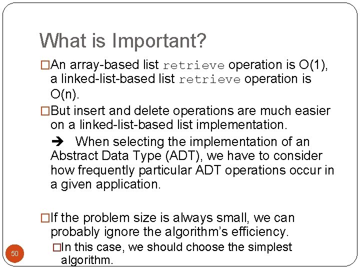
What is Important? �An array-based list retrieve operation is O(1), a linked-list-based list retrieve operation is O(n). �But insert and delete operations are much easier on a linked-list-based list implementation. When selecting the implementation of an Abstract Data Type (ADT), we have to consider how frequently particular ADT operations occur in a given application. �If the problem size is always small, we can probably ignore the algorithm’s efficiency. 50 �In this case, we should choose the simplest algorithm.

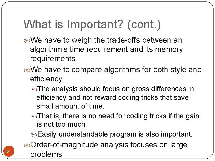
What is Important? (cont. ) We have to weigh the trade-offs between an algorithm’s time requirement and its memory requirements. We have to compare algorithms for both style and efficiency. The analysis should focus on gross differences in efficiency and not reward coding tricks that save small amount of time. That is, there is no need for coding tricks if the gain is not too much. Easily understandable program is also important. 51 Order-of-magnitude analysis focuses on large problems.

Sequential Search int sequential. Search(const int a[], int item, int n){ for (int i = 0; i < n && a[i]!= item; i++); if (i == n) return – 1; return i; } Unsuccessful Search: O(n) Successful Search: Best-Case: item is in the first location of the array O(1) Worst-Case: item is in the last location of the array O(n) Average-Case: The number of key comparisons 1, 2, . . . , n O(n) 52

Binary Search int binary. Search(int a[], int size, int x) { int low =0; int high = size – 1; int mid; // mid will be the index of // target when it’s found. while (low <= high) { mid = (low + high)/2; if (a[mid] < x) low = mid + 1; else if (a[mid] > x) high = mid – 1; else return mid; } return – 1; } 53

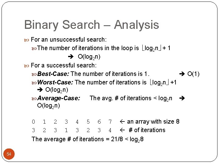
Binary Search – Analysis For an unsuccessful search: The number of iterations in the loop is log 2 n + 1 O(log 2 n) For a successful search: Best-Case: The number of iterations is 1. O(1) Worst-Case: The number of iterations is log 2 n +1 O(log 2 n) Average-Case: The avg. # of iterations < log 2 n O(log 2 n) 0 1 2 3 4 5 6 7 an array with size 8 3 2 3 1 3 2 3 4 # of iterations The average # of iterations = 21/8 < log 28 54