Alexander Tabarrok The Fundamental Problem of Causal Inference

Alexander Tabarrok The Fundamental Problem of Causal Inference
 Yi. T=Outcome for i when T=1 Yi.")
Ideal and Real Data T=Treatment (0, 1) Yi. T=Outcome for i when T=1 Yi. NT=Outcome for i when T=0

What can we Learn from Real Data?

Danger! The average outcome among the treated minus the average outcome among the untreated is not, except under special circumstances, equal to the average treatment effect.

What can we Learn from Real Data? But is interesting? anything
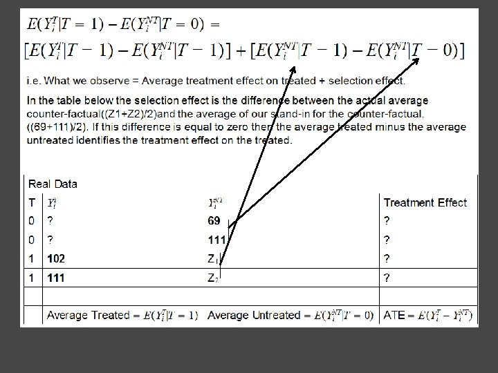

ATE, ATT, ATU Call what we observe the Naïve Average Treatment Effect, NATE. We just showed that NATE=ATT+Selection Effect But what about the ATE? How does this differ from ATT?

Homework I showed NATE=ATT+Selection Effect Write NATE in terms of the ATE. Use ATE, ATT, ATU let p=probability of treatment

The Gold Standard The gold standard is randomization. If units are randomly assigned to treatment then the selection effect disappears. i. e. with random assignment the groups selected for treatment and the groups actually treated would have had the same outcomes on average if not treated. With random assignment the average treated minus the average untreated measures the average treatment effect on the treated (and in fact with random assignment this is also equal to the average treatment effect). In a randomized experiment we select N individuals from the population and randomly split them into two groups the treated with Nt members and the untreated with N-Nt.
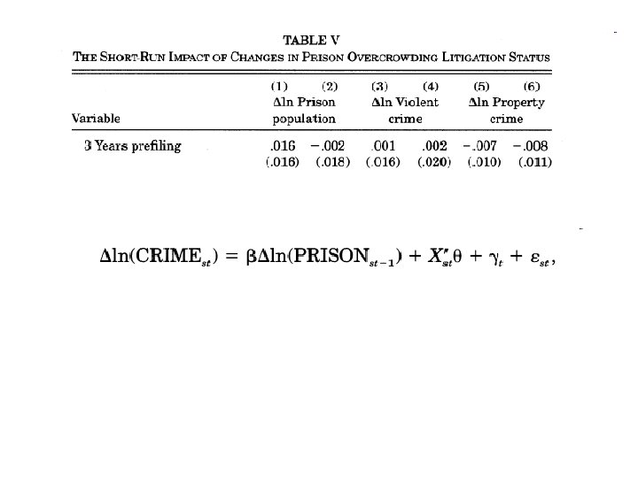
 In a regression context we can run the following regression: and BT")
Regression (Aside) In a regression context we can run the following regression: and BT will measure the treatment effect. It's useful to run through this once in the simple case to prove that this is true. See handout. Bottom line one can prove in this example

Matching Regression is typically one of the first techniques discussed in a class on causal inference but a much more intuitive and straightforward approach is matching. Basic idea: Match on observables then compute statistics such as the ATE.

One Difference Example Suppose we are interested in the effect of a training program on wages. We have data on the wages of trainees and nontrainees. Naïve ATE 11075 -11101. 25=-26. 24 But note that average is higher in non-trainee sample and wages typically increase with age. Let’s match on wages to find the average treatment effect on the treated. (from Cunningham’s Mixtape)

Matched sample. Compare with Treated sample-note age means are identical. ATET on matched sample 11075 -9380=1695.

When can we use matching? Matching methods allow you to construct valid comparison groups when the assignment to the treatment is done on the basis of observable variables. oesn’t Warning: Matching d ias that b n o ti c le e s r fo l o tr n o c nment arises when the assig e on to the treatment is don the basis of nonither observables. (n. b. ne ed IV) does regression. Ne Slide from Gertler et al. World Bank

Matching with More Than One Conditioning Variable If we have more than one conditioning variable, e. g. age and gender then in principle there is no problem, we form matches within each block, calculate a treatment effect within block and form the weighted sum (probability of each block) to get the ATE. A slightly different procedure which fits within a regression context is to use fixed effects for each block (“quasi-matching”).
, 2001, Peer effects with random assignment: Results")
Peer Effects and Matching Sacerdote, B. (Dartmouth), 2001, Peer effects with random assignment: Results for Dartmouth roommates. Quarterly Journal of Economics, 116(2), 681 -704

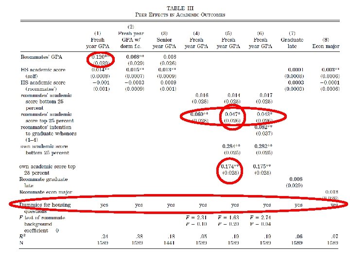
Random within blocks Five questions 1. 2. 3. 4. 5. I smoke. I like to listen to music while studying. I keep late hours. I am more neat than messy. I am male. 5^2=32 blocks (25 non-empty). Within block, assignment is random! For a pure matching estimator, Sacerdote would estimate treatment within blocks. He wants to include some controls, however, and so for efficiency will use dummy variables which we will explain shortly. Similar philosophy to matching.

Show Pre-Treatment Variables are Randomized
 in the roommate’s GPA, a student’s")
Peer Effects For every 1 point increase (decrease) in the roommate’s GPA, a student’s GPA increased (decreased) about. 12 points. If you would have been a 3. 0 student with a 3. 0 roommate, but you were assigned to a 2. 0 roommate, your GPA would be 2. 88. Note that the peer effect in ability is 27% as large as the own effect! Peer effects are even larger in social choices such as the choice to join a fraternity. (Dorm effects are large here as well. )

Random within blocks In the case of the Dartmouth experiment we knew that residents were matched randomly within the blocks so we just had to control for the block. An exact match. But typically, when there are multiple conditioning variables we won’t be able to find exact matches.

The Curse of Dimensionality Matching breaks down when we add covariates. E. g. Suppose that we have two variables each with 10 levels, then we need 100 cells and we need treated and untreated members of each cell. Add one more 10 level variable and we need 1000 cells. Regression “solves” this problem by imposing linear relationships e. g. Y=α + β 1 PSA + β 2 Age + β 3 Age × PSA + β 4 T We have reduced (squashed!) a 100 variable problem to 3 variables but at the price of assuming away most of the possible variation.

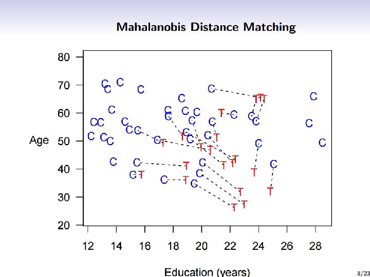
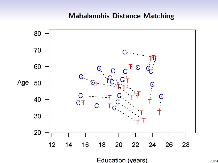
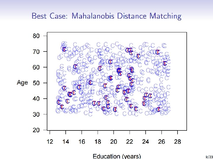
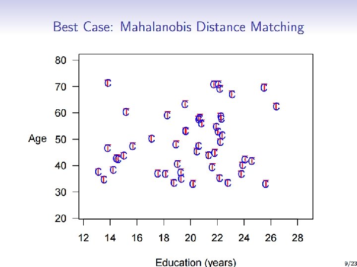
Distance Measures If we can’t do exact matching then we can match observations according to how “close” the are. But how to measure closeness or distance? Mahalanobis Propensity Score Coarsened

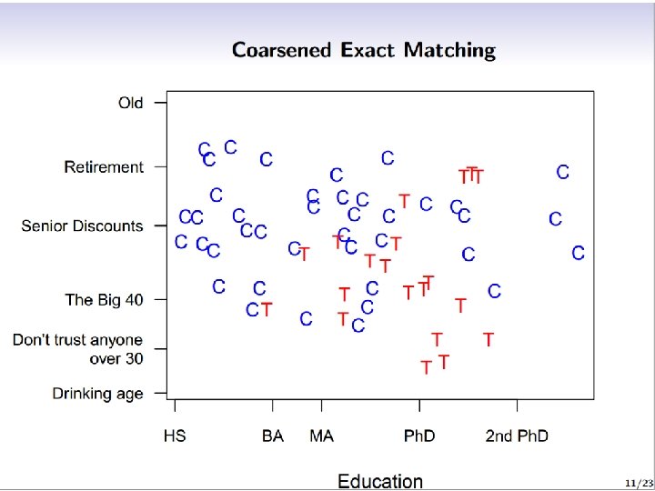
Slides from Gary King

lso a d l u g co n i h ing t c t a a n i m elim hat > t e g t n o i on N un m r p m o d c e l be cal s not in the le variab. rt suppo
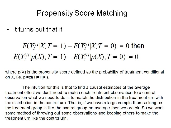

Matching based on the Propensity Score Definition The propensity score is the conditional probability of receiving the treatment given the pre-treatment variables: p(X) =Pr{T = 1|X} = E{T|X} Lemma 1 If p(X) is the propensity score, then T X | p(X) “Given the propensity score, the pre-treatment variables are balanced between beneficiaries and non- beneficiaries” Lemma 2 Y 1, Y 0 T | X => Y 1, Y 0 T | p(X) “Suppose that assignment to treatment is unconfounded given the pre-treatment variables X. Then assignment to treatment is unconfounded given the propensity score p(X). ”

Does the propensity score approach solve the dimensionality problem? YES! The balancing property of the propensity score (Lemma 1) ensures that: o Observations with the same propensity score have the same distribution of observable covariates independently of treatment status; and o for a given propensity score, assignment to treatment is “random” and therefore treatment and control units are observationally identical on average.

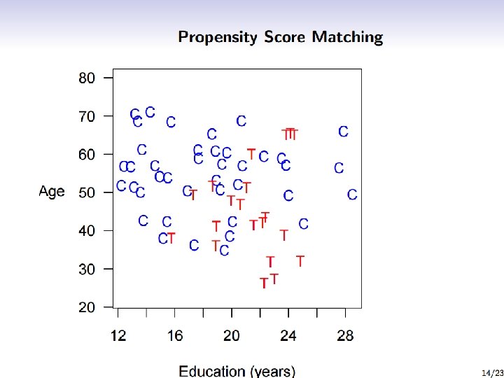
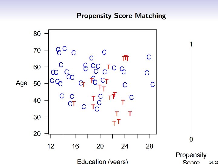
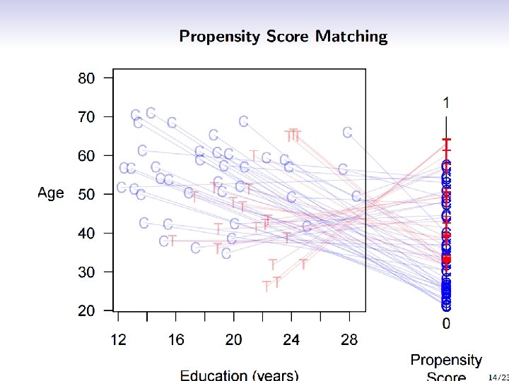
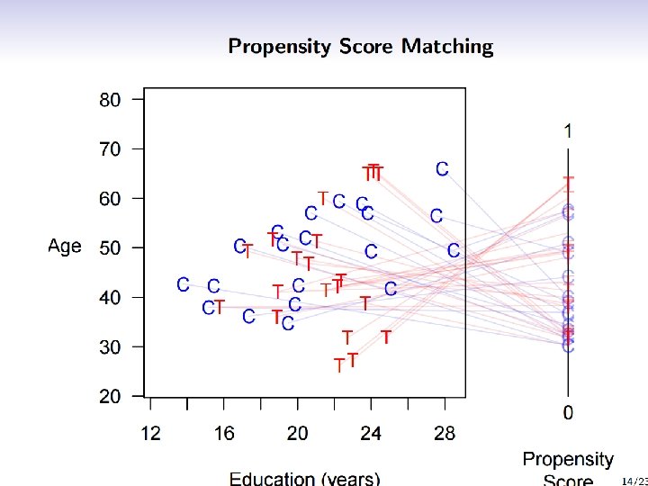
The Philosophy of PS Matching

Implementation of the estimation strategy Remember we’re discussing a strategy for the estimation of the average treatment effect on the treated, called δ Step 1 Estimate the propensity score (e. g. logit or probit) Step 2 Estimate the average treatment effect given the propensity score o o o match treated and controls with “nearby” propensity scores compute the effect of treatment for each value of the (estimated) propensity score obtain the average of these conditional effects

Step 2: Estimate the average treatment effect given the propensity score The closest we can get to an exact matching is to match each treated unit with the nearest control in terms of propensity score “Nearest” can be defined in many ways. These different ways then correspondent to different ways of doing matching: o o o Stratification on the Score Nearest neighbor matching on the Score Weighting on the basis of the Score

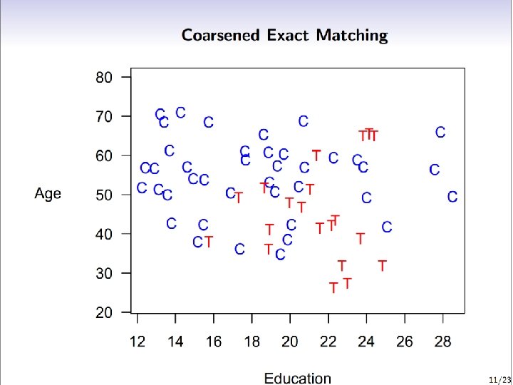
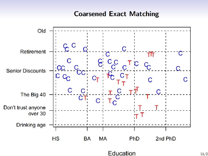
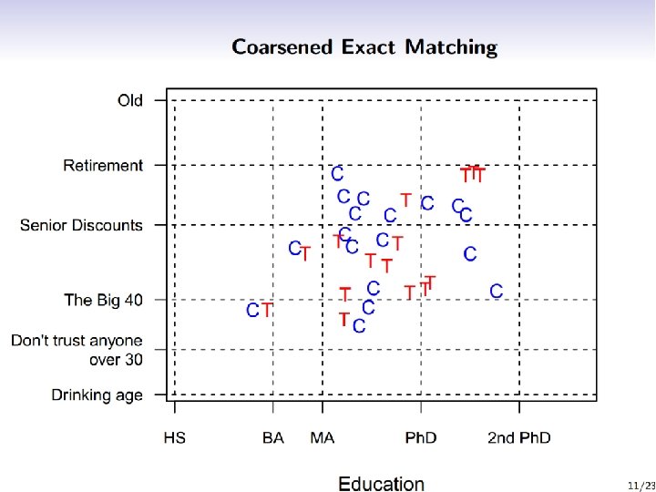
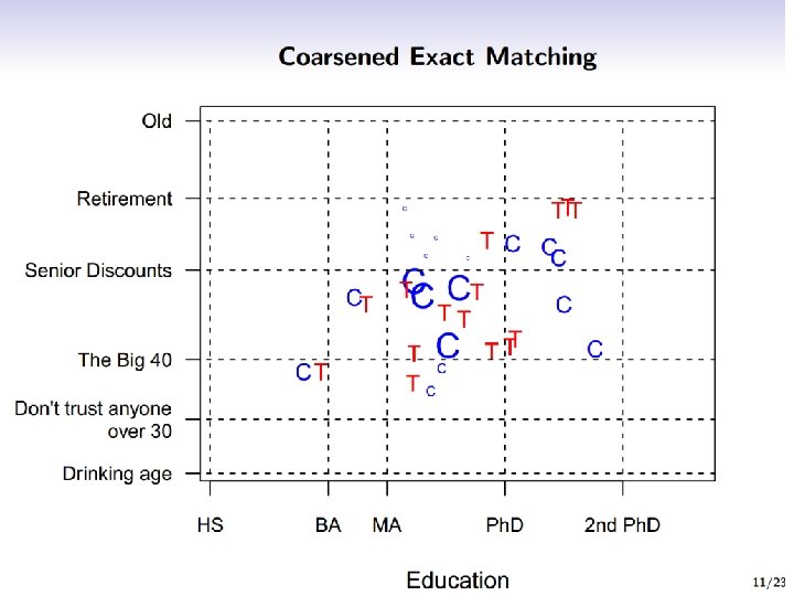
ything r e v e zing e e u q te: S ses o o l n n e o i d hing c Si ns t e a m m i d e nce into on ion so dista g work at in inform ened match g). n i K y s r r or coa general (Ga in better

es prun g n i h matc t a h t note n i a g A ions. t a v r e s the ob
")
Matching Methods Stata o Nearest neighbor matching using Mahalanobis metric teffects nnmatch (y x) (t), atet o Propensity score matching using logit teffects psmatch (y) (t x, logit), atet o Propensity Score Matching using PSMatch 2 psmatch 2 t x, outcome(y) o Coarsened Exact Matching cem x (cutpoints/cutalgorithm), treatment(t)

Inverse Probability Weighting Rather than matching 1 to 1 it is possible to match one treated to all untreated but adjusting the weights on the untreated to account for similarity. Uses more data and is also unbiased. When the objective is to estimate ATET, the treated person receives a weight of 1 while the control person receives a weight of p(X)/(1 -p(X)).

Propensity Score Matching as Diagnostic and Explanatory Tool

The circle labeled "earnings" illustrates variation in the variable to be explained. Education and Ability are correlated explanatory variables and Ability is not observed. The blue area within the instrument circle represents variation in education that is uncorrelated with Ability and which can be used to consistently estimate the coefficient on education. Note that the only reason the instrument is correlated with Earnings is through education.

Angrist-Krueger IV Cunningham, Mixtape. Children born in December and children born in January are similar but at around age 6 the former goes to school and the latter is still in kindergarten. Either, however, can quit at age 16 but the December quitter will have had more school at age 16 than the January (1’st QOB) quitter.
")
Instruments in Action (Angrist and Krueger 1991)

Instrumental variables with weak instruments and correlation with unobserved influences. Bias in the IV estimator is determined by the covariance of the instrument with education (blue within instrument circle) relative to the covariance between the instrument and the unobserved factors (red within instrument circle). Thus IV with weak instruments can be more biased than OLS.

Voluntary job training program Say we decide to compare outcomes for those who participate to the outcomes of those who do not participate: A simple model to do this: y = α + β 1 P + β 2 x + ε P= 1 0 If person participates in training If person does not participate in training x = Control variables (exogenous & observed) Why is this not working? 2 problems: o Variables that we omit (for various reasons) but that are important o Decision to participate in training is endogenous.

Problem #1: Omitted Variables Even if we try to control for “everything”, we’ll miss: (1) Characteristics that we didn’t know they mattered, and (2) Characteristics that are too complicated to measure (not observables or not observed): o Talent, motivation o Level of information and access to services o Opportunity cost of participation Full model would be: y = γ 0 + γ 1 x + γ 2 P + γ 3 M 1 + η But we cannot observe M 1 , the “missing” and unobserved variables.

Omitted variable bias True model is: y = γ 0 + γ 1 x + γ 2 P + γ 3 M 1 + η But we estimate: y = β 0 + β 1 x + β 2 P + ε If there is a correlation between M 1 and P, then the OLS estimator of β 2 will not be a consistent estimator of γ 2, the true impact of P. Why? When M 1 is missing from the regression, the coefficient of P will “pick up” some of the effect of M 1

Problem #2: Endogenous Decision to Participate True model is: y = γ 0 + γ 1 x + γ 2 P + η with P = π0 + π 1 x + π 2 M 2 +ξ M 2 = Vector of unobserved / missing characteristics (i. e. we don’t fully know why people decide to participate) Since we don’t observe M 2 , we can only estimate a simplified model: y = β 0 + β 1 x + β 2 P + ε Is β 2, OLS an unbiased estimator of γ 2?

Problem #2: Endogenous Decision to Participate We estimate: y = β 0 + β 1 x + β 2 P + ε But true model is: y = γ 0 + γ 1 x + γ 2 P + η with P = π0 + π1 x + π2 M 2 +ξ Is β 2, OLS an unbiased estimator of γ 2? Corr (ε, P) = corr (ε, π 0 + π 1 x + π 2 M 2 +ξ) = π 1 corr (ε, x)+ π 2 corr (ε, M 2) = π 2 corr (ε, M 2) If there is a correlation between the missing variables that determine participation (e. g. Talent) and outcomes not explained by observed characteristics, then the OLS estimator will be biased.

What can we do to solve this problem? We estimate: y = β 0 + β 1 x + β 2 P + ε So the problem is the correlation between P and ε How about we replace P with “something else”, call it Z: o Z needs to be similar to P o But is not correlated with ε

Back to the job training program P = participation ε = that part of outcomes that is not explained by program participation or by observed characteristics I’m looking for a variable Z that is: (1) (2) Closely related to participation P but doesn’t directly affect people’s outcomes Y, other than through its effect on participation. So this variable must be coming from outside.

Generating an outside variable for the job training program Say that a social worker visits unemployed persons to encourage them to participate. o She only visits 50% of persons on her roster, and o She randomly chooses whom she will visit If she is effective, many people she visits will enroll. There will be a correlation between receiving a visit and enrolling But visit does not have direct effect on outcomes (e. g. income) apart from its effect through enrollment in the training program. Randomized “encouragement” or “promotion” visits are an Instrumental Variable.

Characteristics of an instrumental variable Define a new variable Z Z= 1 If person was randomly chosen to receive the encouragement visit from the social worker 0 If person was randomly chosen not to receive the encouragement visit from the social worker Corr ( Z , P ) > 0 People who receive the encouragement visit are more likely to participate than those who don’t Corr ( Z , ε ) = 0 No correlation between receiving a visit and benefit to the program apart from the effect of the visit on participation. Z is called an instrumental variable


Extra

Matching
- Slides: 74