Aleatory and Epistemic Uncertainties in Interpolated Ground Motions

Aleatory and Epistemic Uncertainties in Interpolated Ground Motions Example from the Kashiwazaki-Kariwa Nuclear Power Plant Recordings of the July 16, 2007, Niigataken Chuetsu-oki, Japan, Earthquake Antonella Cirella 1, Paul Spudich 2 1 INGV, Rome, Italy 2 USGS, Menlo Park, CA EGU 2013, SM 2. 5, 5932, Vienna

Using an earthquake rupture model to ‘predict’ ground motions at unobserved locations When earthquake occur, we could have a few recordings of ground motion, but not a sites where something interesting and /or bad occurred. (e. g. 2007 Niigata-ken Chuetsu-oki) EGU 2013, SM 2. 5, 5932, Vienna

Using an earthquake rupture model to ‘predict’ ground motions at unobserved locations Post-Earthquake forensic studies and ‘Shake-Map’ generation rely upon ground-motion interpolation (process to infer, from a set of ground motions, observed at sparse observation locations, the ground motion at a target site where no observation were made during the earthquake) EGU 2013, SM 2. 5, 5932, Vienna

Using an earthquake rupture model to ‘predict’ ground motions at unobserved locations It is now possible to invert observed ground motions to obtain the spatiotemporal behavior of rupture on the causative fault Forward predict ground motions (SA) at unobserved locations But the inversion is inherently non-unique Ø How large is the scatter in the interpolated ground motions? Ø Is the scatter of the predicted motions large enough to include the true motions at the target sites? Ø Is the scatter of the predicted motions at the unobserved site larger than the scatter of the predicted motions at sites having data used in the inversion? Ø What controls the level of error? EGU 2013, SM 2. 5, 5932, Vienna

A problem in linear inference, except… • Theoretically, the process of ground-motion interpolation is an example of linear inference. • For a linear problem lacking bounds on the model space, the interpolated ground motion can be completely unbounded. • When bounds like positivity and known moment are added as constraints on the model, the interpolated motions may then become bounded, and could be explored using algorithm BVLS of Stark and Parker (1995), which can compute bounds on linear functionals of an inverted model. • However, the response spectrum is a nonlinear function of the ground acceleration time series, and consequently we have chosen to investigate the variability of interpolated response spectra using a statistical approach building on a non-linear inversion method (Piatanesi et al, 2007; Cirella et al, 2008) EGU 2013, SM 2. 5, 5932, Vienna

Kinematic Inversion Technique Ø joint and separate inversion of strong motion, GPS and DIn. SAR data; Ø finite fault is divided into sub-faults; Ø Ø kinematic parameters are allowed to vary within a sub-fault; Heat-Bath Simulated Annealing algorithm; Output of kinematic inversion: Model Ensemble Ω = Inverted Parameters: • Peak Slip Velocity; • Rise Time; • Rupture Time; • Rake. Rupture Models m & Cost Function C(m) EGU 2013, SM 2. 5, 5932, Vienna

Kinematic Inversion: 2007 Niigata-ken Chuetsu-oki Earthquake, Mw=6. 6 § 13 stations (surface or borehole strong motion records); § 15 GPS stations ; § frequency-band: (0. 0÷ 0. 5)Hz; § 60 sec (body & surface waves); § all kinematic parameters are inverted simultaneously. EGU 2013, SM 2. 5, 5932, Vienna

EGU 2013, SM 2. 5, 5932, Vienna

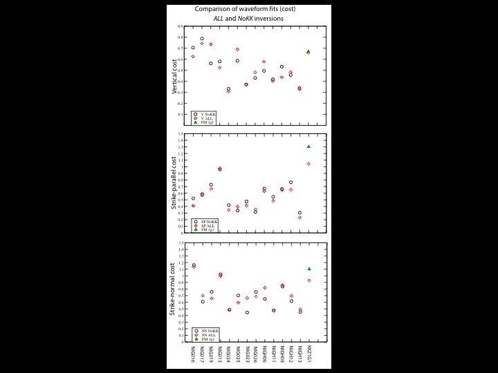
Cost function for the inversion not using KK data 4% above min cost – 8561 models 3 % above min cost – 4897 models 2% above min cost – 1534 models 1% above min cost – 334 models 0. 5% above min cost – 122 models EGU 2013, SM 2. 5, 5932, Vienna min cost - best fitting model

Waveforms fit for the 4% model ensemble are not obviously worse than for the 1% ensemble. Different rupture models can fit the observed data equally well, due to the intrinsic nonuniqueness of the inversion. EGU 2013, SM 2. 5, 5932, Vienna

Bias as the ratio of the observed response spectrum to the synthetic as a function of period. 5% SA Bias (epistemic error) Aleatory error – Nonunique prediction scatter Biases at 2 -3 s bigger than nonunique prediction scatter EGU 2013, SM 2. 5, 5932, Vienna quantifies the scatter in the predicted spectral acceleration Form of aleatory uncertainty in the ground motion prediction due to unknown aspects of slip distributions. (data from future EQs will not reduce the uncertainty of this ground motion prediction for this past earthquake)

For a true interpolation of a ground motion where there is no observation, the horizontal scatter can be at least 20 -25% bigger than the scatter predicted from good fitting models at sites with observed motions. 22% These results are unaffected by the characteristic of the 1 g 1 data (not used in the inversion!) EGU 2013, SM 2. 5, 5932, Vienna

Comparison of nonunique prediction scatter with aleatory sigma from kinematic and dynamic rupture simulations of ground motions kinematic rupture models contain generate variability too much source variability (real by using 2 groups randomly simulate ahave M 6. 5 ofcorrelated strike-slip earthquake ruptures variable initial)stress and a M 6. 5 dip-slip at aleatory variability inquake ground source properties distributions, input into different sites, adopting motions calculated for Variability of by predicted dynamic rupture different slip distributions kinematic rupture models ground motion forsimulations a M 6. 5, and by to generate variable slip different hypocenters. theoretical Green's functions considering uncertainties on models, fixed andof EGF’ eventwith & variability variable hypo, from which source properties ground motions at different were generated. A&Ssites 2008 Intra-event the correlations of source properties in dynamic models do result in lower ground motion variability A&S 2008 inter-event scatter in the predictions due to the nonuniqueness of our non-uniqueness scatter at 1 g 1 for the 4% model ensemble approaches ‘good’ rupture the Abrahamson and Silva’s observed inter-event scatter. This means that models the non-uniqueness variability of predicted motion at 1 g 1 is almost as great as the variability of motion incurred by using a different earthquake having the same magnitude and hypocenter to predict the motion at 1 g 1. EGU 2013, SM 2. 5, 5932, Vienna

Conclusions ü We computed the scatter in predictions of SA at 1 g 1 based on the nonuniqueness of inverted kinematic rupture models of the 2007 Niigata-ken Chuetsu-oki earthquake. ü The scatter in the predicted horizontal response spectra at 1 g 1 from the inversion is is about 22% bigger than the scatter of response spectra predicted at the Niigata stations. This result says, that in the case of a true interpolation of a ground motion where there is no observation, the scatter in the horizontal component interpolant can be 20 -25% bigger than the scatter in the motions predicted from good fitting models at sites where there were observed motions. ü We compared our nonuniqueness scatter with aleatory variation of ground motions from kinematic and dynamic rupture models: q aleatory scatter values of the ground motions from kinematic rupture models exceed the empirically observed scatter in response spectra from a standard GMPE (Abrahamson and Silva, 2008), excluding the effects of variable soil amplification. Clearly these kinematic rupture models contain too much source variability; EGU 2013, SM 2. 5, 5932, Vienna

q the aleatory variation of dynamic rupture ground motions is much smaller than that of the kinematic rupture models, indicating that the correlations of source properties in dynamic models result in lower ground motion variability; q our non-uniqueness scatter at 1 g 1 approaches Abrahamson and Silva’s observed interevent scatter. This means that the variability of predicted motion at 1 g 1 caused by nonuniqueness in the rupture model is almost as great as the variability of motion incurred by using a different earthquake having the same magnitude and hypocenter to predict the motion at 1 g 1. While the bias of interpolated ground motions has not been our main topic of investigation, the biases are of first order importance in the estimation of ground motion at a particular site using interpolation of motion from surrounding stations. The nonunique prediction scatter is a hitherto uninvestigated source of aleatory variability that should be included in studies of aleatory variability which use observed slip distributions with randomized hypocenters. Spudich P. and A. Cirella. , “Aleatory and Epistemic Uncertainties in Interpolated Ground Motions- Example from the Kasiwasaki-Kariwa Nuclear Power Plant recordings of the July 16, 2007 Niigata-ken Chuetsu-oki, Japan, Earthquake”, , submitted to Bulletin of the Seismological Society of America. EGU 2013, SM 2. 5, 5932, Vienna

Acknowledgements • Accelerograms from the KKNPP were provided by the Association of Earthquake Disaster Prevention, Tokyo, Japan, which is the sole distributor of such data. Copyright of all KKNPP data belongs to the Tokyo Electric Power Company. • We thank Dr. Kenishi Tsuda of Shimizu Corporation for providing insight into sources of information for this study, and we thank Drs. Arben Pitarka and Enrico Priolo for providing unpublished supplementary materials. • This work was supported by the U. S. Nuclear Regulatory Commission (NRC) Office of Research Job Code N 6501. Spudich P. and A. Cirella. , “Aleatory and Epistemic Uncertainties in Interpolated Ground Motions- Example from the Kasiwasaki-Kariwa Nuclear Power Plant recordings of the July 16, 2007 Niigata-ken Chuetsu-oki, Japan, Earthquake”, , submitted to Bulletin of the Seismological Society of America. EGU 2013, SM 2. 5, 5932, Vienna

THE END

Supplementary Material. Modelli Invertiti con & senza kkp con relativi fit figure 7 e 8. Confronto valori di cost function: figure 9. Formule SA(T=2 sec); . Formule scatter, bias. . Confronto con gli altri lavori: figure necessarie EGU 2013, SM 2. 5, 5932, Vienna

Kinematic Inversion Technique Stage I: Building Model Ensemble-HB Simulated Annealing START random model m 0 Loop over temperatures Loop over iterations Loop over parameters (Vr, …) Loop over model values Forward Modeling: Compsyn Misfit computation end end Simulated annealing Heat-bath algorithm To quantify the misfit… C(m) Strong = motion + L 1+L 2 norm GPS L 2 norm EGU 2013, SM 2. 5, 5932, Vienna + DIn. SAR L 2 norm

Kinematic Inversion Technique Stage II: Appraisal of the Ensemble Output of kinematic inversion: Ω Model Ensemble Ω = Rupture Models m & Cost Function C(m) Ø Best Model Ø Average Model: Ø Standard Deviation: EGU 2013, SM 2. 5, 5932, Vienna

Kinematic Inversion: 2007 Niigata-ken Chuetsu-oki Earthquake, Mw=6. 6 § 13 stations (surface or borehole strong motion records); § 15 GPS stations ; § frequency-band: (0. 02÷ 0. 5)Hz; § 60 sec (body & surface waves); § South-East Dipping Fault; § W=31. 5 km; L=38. 5 km; =3. 5 km; § all kinematic parameters are inverted simultaneously. July 16 -th 2007

Best Model: E(m)=0. 3 Average Model: E(m)=0. 4 • The best fitting model might contain an extreme configuration of model parameters; n The ensemble-averaged model better represents the stable features of the rupture history.

Comparison between synthetics (red) and observed (blue) waveforms. GPS Comparison between synthetics (white) and observed (red) coseismic horizontal displacement. Strong Motion

EGU 2013, SM 2. 5, 5932, Vienna

Formula SA EGU 2013, SM 2. 5, 5932, Vienna

EGU 2013, SM 2. 5, 5932, Vienna

Comparison of nonunique prediction scatter with aleatory sigma from kinematic and dynamic rupture simulations of ground motions EGU 2013, SM 2. 5, 5932, Vienna

Results 1. Almost all of the aleatory scatter values of the ground motions from kinematic rupture models exceed the blue dashed line, which is the empirically observed scatter in response spectra, excluding the effects of variable soil amplification. Clearly these kinematic rupture models contain too much source variability. Abrahamson (personal communication) has speculated that real earthquake ruptures have correlated source properties (for example, local rupture velocity and peak slip velocity at the same point, for example) that are not present in the kinematic rupture models, leading to excessive variation in the kinematic rupture models and resulting ground motion. 2. The aleatory variation of Ripperger’s ground motions is much smaller than that of the kinematic rupture models, indicating that the correlations of source properties in dynamic models do result in lower ground motion variability, although we must bear in mind that Ripperger’s variability of stress drop is less than a factor of two, in other words, rather low. 3. Ripperger’s variability is comparable to the empirical variability. Abrahamson and Silva’s blue dashed line includes the effects of variable source properties (for example, stress drop) as well as variations like directivity amplification that vary from site to site in a single earthquake. Ripperger’s variability for variable hypocenter location agrees rather well with the blue dashed line. However, Ripperger’s result for fixed hypocenter is a bit bigger than the empirically observed earthquake-to-earthquake variation (red dashed line), despite Ripperger’s rather small stress drop variation. 4. Our nonuniqueness scatter at 1 g 1 for the 4% model ensemble approaches Abrahamson and Silva’s observed interevent scatter. This means that the nonuniqueness variability of predicted motion at 1 g 1 is almost as great as the variability of motion incurred by using a different earthquake having the same magnitude and hypocenter to predict the motion at 1 g 1. (We make the ‘same hypocenter’ restriction because differences in directivity contribute to the intraevent error that is characterized by the ‘total’ sigma curve in the figure. ) Of course, this observation depends on the choice of the 4% ensemble which is arbitrary. 5. Spectral acceleration predictions based on ground motion inversions and dynamic simulations might be less accurate than simply predicting the spectral acceleration from a GMPE such as Abrahamson and Silva (2008) with a directivity correction (for example, Somerville et al. , 1997). (Or maybe the GMPE sigma is too small? ) EGU 2013, SM 2. 5, 5932, Vienna