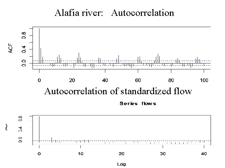
Alafia river Autocorrelation of standardized flow Alafia River

Alafia river: Autocorrelation of standardized flow

Alafia River: Monthly streamflow distribution

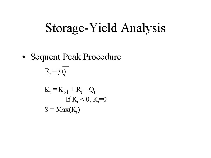
Storage-Yield Analysis • Sequent Peak Procedure Rt = y Kt = Kt-1 + Rt – Qt If Kt < 0, Kt=0 S = Max(Kt)

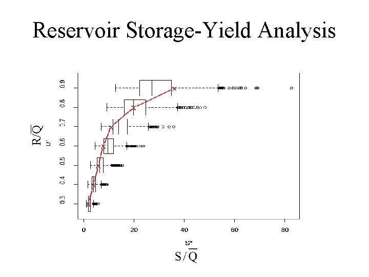
R/Q Reservoir Storage-Yield Analysis

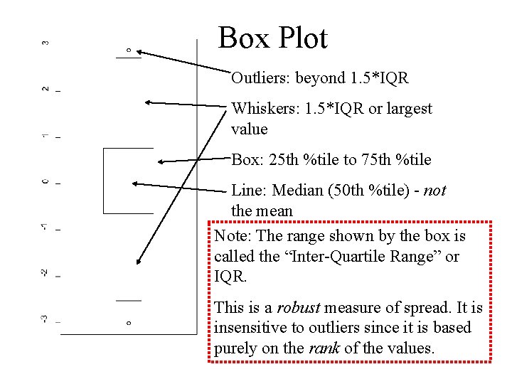
Box Plot Outliers: beyond 1. 5*IQR Whiskers: 1. 5*IQR or largest value Box: 25 th %tile to 75 th %tile Line: Median (50 th %tile) - not the mean Note: The range shown by the box is called the “Inter-Quartile Range” or IQR. This is a robust measure of spread. It is insensitive to outliers since it is based purely on the rank of the values.

Reservoir Reliability Analysis

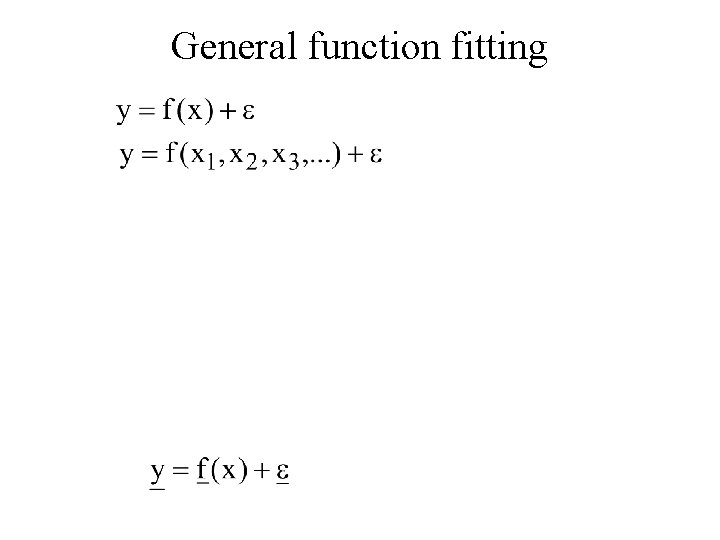
General function fitting

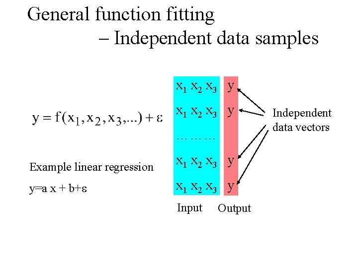
General function fitting – Independent data samples x 1 x 2 x 3 y ……… Example linear regression x 1 x 2 x 3 y y=a x + b+ x 1 x 2 x 3 y Input Output Independent data vectors

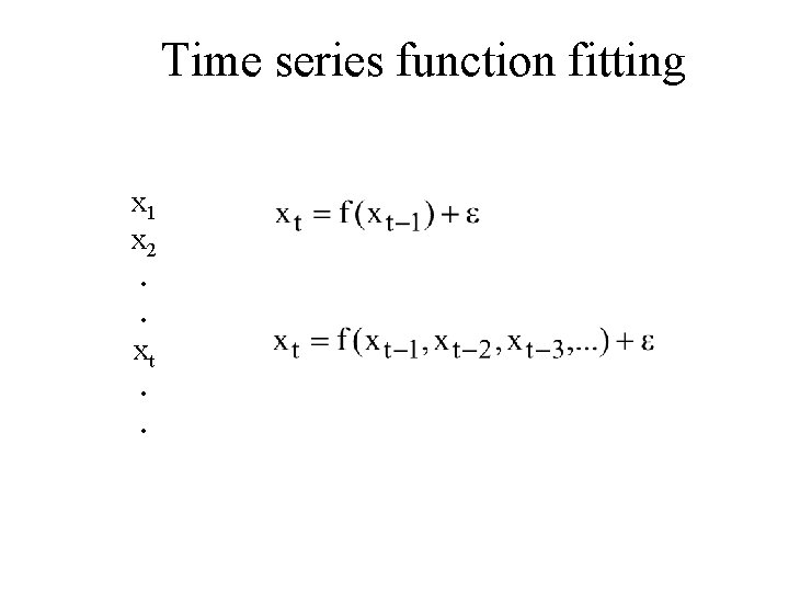
Time series function fitting x 1 x 2. . xt. .

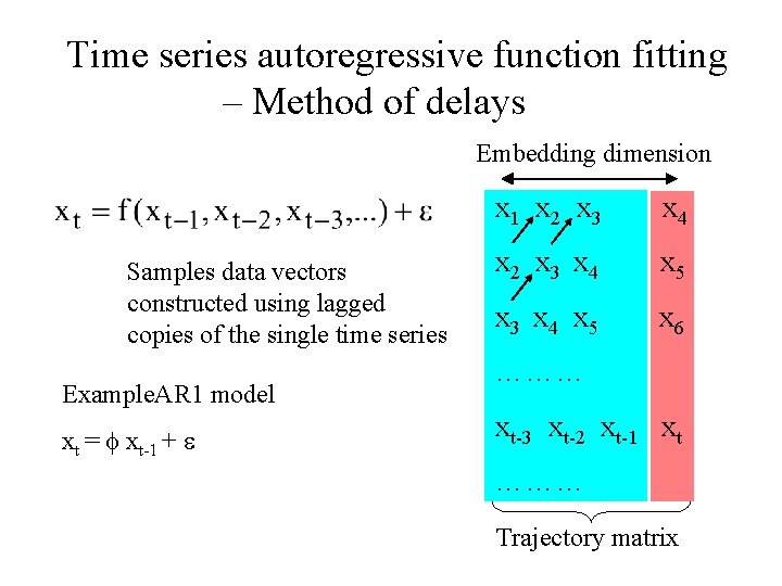
Time series autoregressive function fitting – Method of delays Embedding dimension Samples data vectors constructed using lagged copies of the single time series Example. AR 1 model xt = xt-1 + x 1 x 2 x 3 x 4 x 5 x 6 ……… xt-3 xt-2 xt-1 xt ……… Trajectory matrix

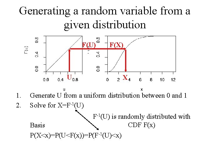
Generating a random variable from a given distribution F(U) F(X) U 1. 2. X Generate U from a uniform distribution between 0 and 1 Solve for X=F-1(U) is randomly distributed with CDF F(x) Basis P(X<x)=P(U<F(x))=P(F-1(U)<x)

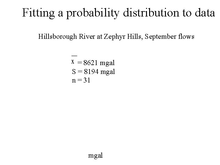
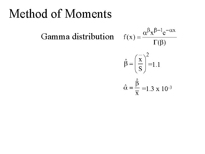
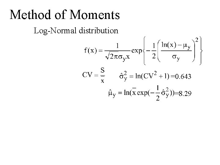
Fitting a probability distribution to data Hillsborough River at Zephyr Hills, September flows = 8621 mgal S = 8194 mgal n = 31 mgal

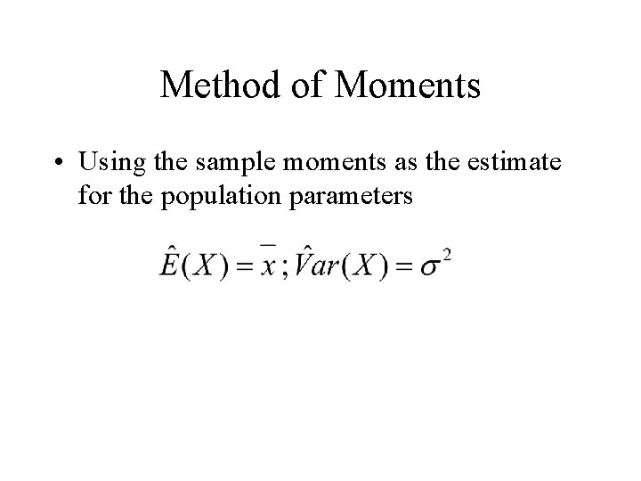
Method of Moments • Using the sample moments as the estimate for the population parameters

Method of Moments Gamma distribution =1. 1 =1. 3 x 10 -3

Method of Moments Log-Normal distribution =0. 643 =8. 29

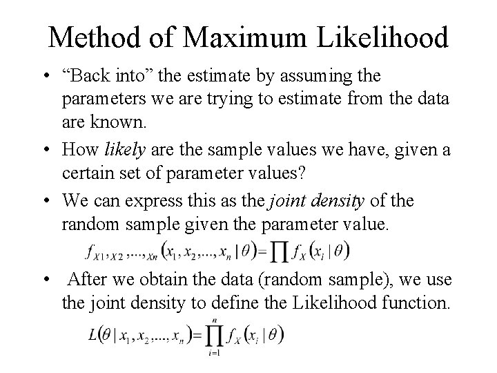
Method of Maximum Likelihood • “Back into” the estimate by assuming the parameters we are trying to estimate from the data are known. • How likely are the sample values we have, given a certain set of parameter values? • We can express this as the joint density of the random sample given the parameter value. • After we obtain the data (random sample), we use the joint density to define the Likelihood function.

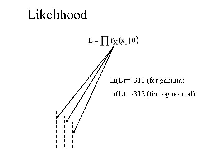
Likelihood ln(L)= -311 (for gamma) ln(L)= -312 (for log normal)

Normalizing Transformations and fitting a marginal distribution • Much theory relies on the central limit theorem so applies to Normal Distributions • Where the data is not normally distributed normalizing transformations are used – Log – Box Cox (Log is a special case of Box Cox) – A specific PDF, e. g. Gamma – A non parametric PDF

Approach • Select the class of distributions you want to fit • Estimate parameters using an appropriate goodness of fit measure – Likelihood – PPCC (Filliben’s statistic) – Kolmogorov Smirnov p value – Shapiro Wilks W

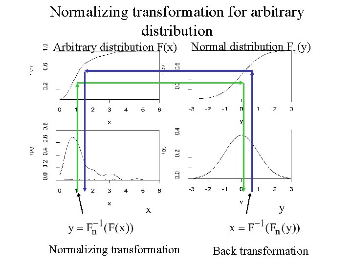
Normalizing transformation for arbitrary distribution Arbitrary distribution F(x) x Normalizing transformation Normal distribution Fn(y) y Back transformation

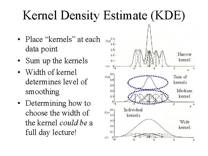
Kernel Density Estimate (KDE) • Place “kernels” at each data point • Sum up the kernels • Width of kernel determines level of smoothing • Determining how to choose the width of the kernel could be a full day lecture! Narrow kernel Sum of kernels Medium kernel Individual kernels Wide kernel

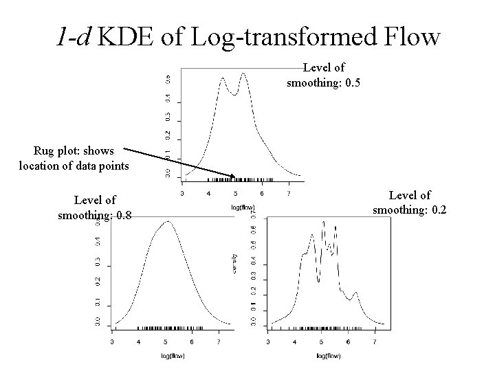
1 -d KDE of Log-transformed Flow Level of smoothing: 0. 5 Rug plot: shows location of data points Level of smoothing: 0. 8 Level of smoothing: 0. 2

Non parametric PDF in R hist(x, nclass=15, main= month. name[i] , xlab="cfs", probability=T) lines(density(x, bw="nrd 0", na. rm=TRUE), col=2) rug(x, , 2)

Non parametric CDF in R cdf. r=function(density) { x=density$x yt=cumsum(density$y) n=length(yt) y=(yt-yt[1])/(yt[n]-yt[1]) # force onto the range 0, 1 without checking for significant error list(x=x, y=y) } dd=density(x, bw="nrd 0", na. rm=TRUE) cdf=cdf. r(dd) plot(cdf, type="l") ylookup. r=function(x, cdf) xlookup. r=function(y, cdf) { int=sum(cdf$y<y) # This identifies the interval for interpolation x=((y-cdf$y[int])*cdf$x[int+1]+(cdf$y[int+1]-y)*cdf$x[int])/(cdf$y[int+1]-cdf$y[int]) return(x) }

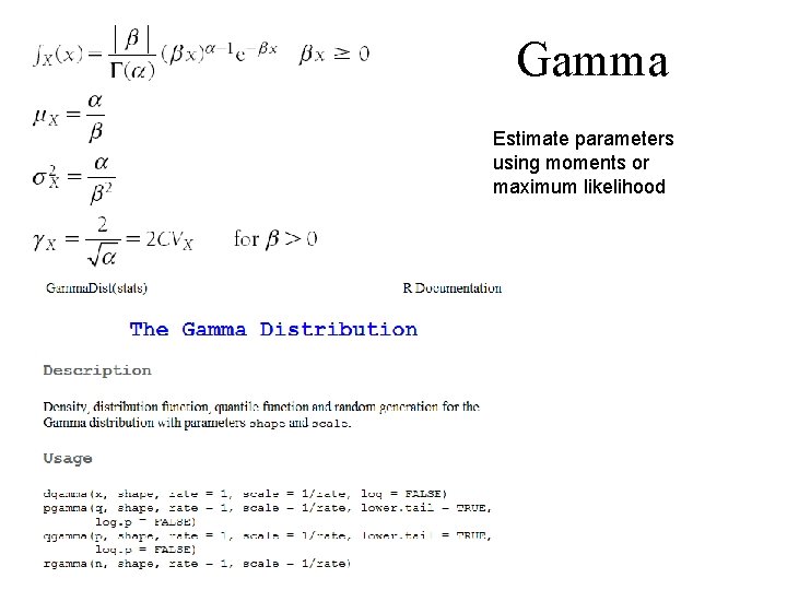
Gamma Estimate parameters using moments or maximum likelihood

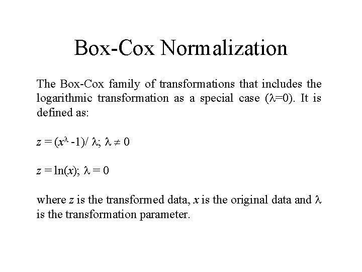
Box-Cox Normalization The Box-Cox family of transformations that includes the logarithmic transformation as a special case ( =0). It is defined as: z = (x -1)/ ; 0 z = ln(x); = 0 where z is the transformed data, x is the original data and is the transformation parameter.

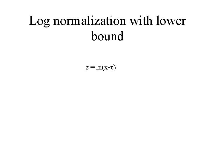
Log normalization with lower bound z = ln(x- )

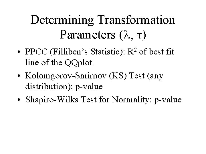
Determining Transformation Parameters ( , ) • PPCC (Filliben’s Statistic): R 2 of best fit line of the QQplot • Kolomgorov-Smirnov (KS) Test (any distribution): p-value • Shapiro-Wilks Test for Normality: p-value

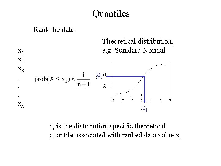
Quantiles Rank the data x 1 x 2 x 3. . . xn Theoretical distribution, e. g. Standard Normal pi qi qi is the distribution specific theoretical quantile associated with ranked data value xi

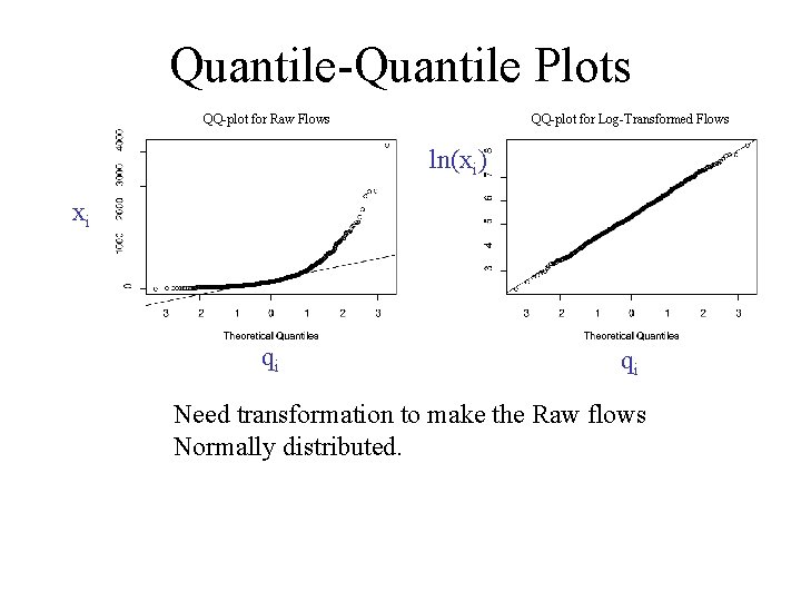
Quantile-Quantile Plots QQ-plot for Raw Flows QQ-plot for Log-Transformed Flows ln(xi) xi qi qi Need transformation to make the Raw flows Normally distributed.

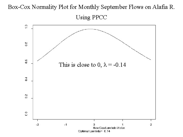
Box-Cox Normality Plot for Monthly September Flows on Alafia R. Using PPCC This is close to 0, = -0. 14

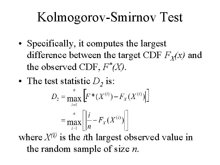
Kolmogorov-Smirnov Test • Specifically, it computes the largest difference between the target CDF FX(x) and the observed CDF, F*(X). • The test statistic D 2 is: where X(i) is the ith largest observed value in the random sample of size n.

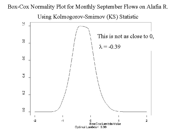
Box-Cox Normality Plot for Monthly September Flows on Alafia R. Using Kolmogorov-Smirnov (KS) Statistic This is not as close to 0, = -0. 39

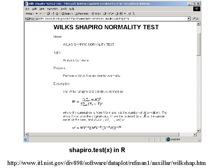
shapiro. test(x) in R http: //www. itl. nist. gov/div 898/software/dataplot/refman 1/auxillar/wilkshap. htm

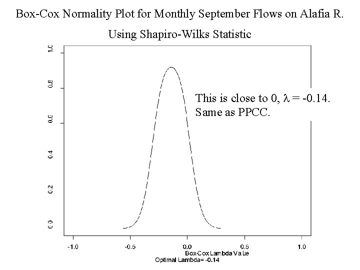
Box-Cox Normality Plot for Monthly September Flows on Alafia R. Using Shapiro-Wilks Statistic This is close to 0, = -0. 14. Same as PPCC.

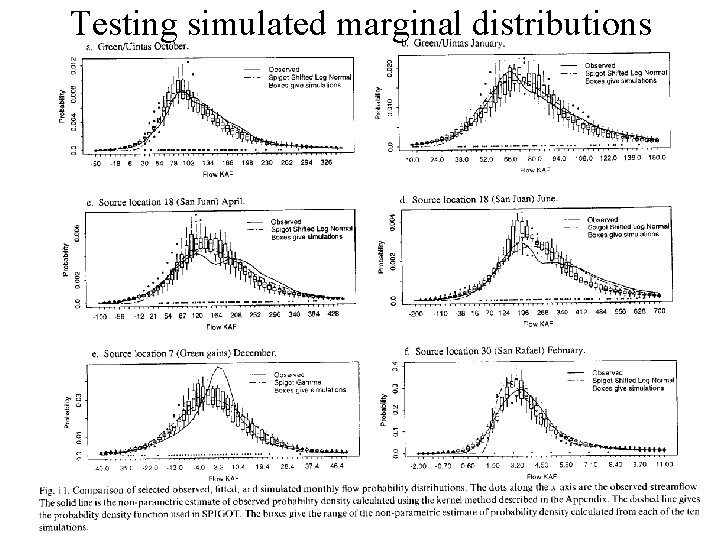
Testing simulated marginal distributions

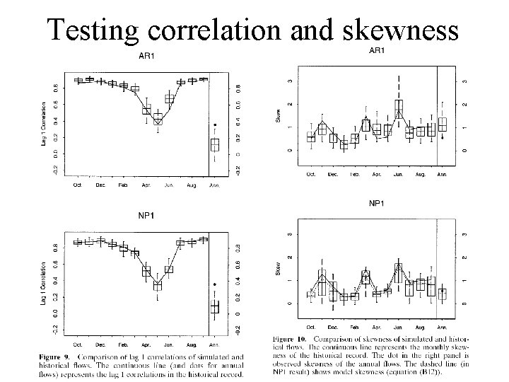
Testing correlation and skewness

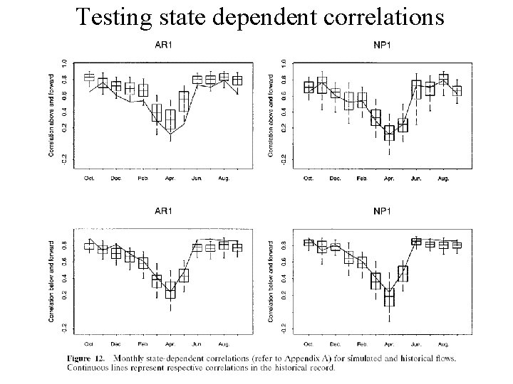
Testing state dependent correlations