Agricultural Economics Lecture 3 Government Intervention in Agriculture

Agricultural Economics Lecture 3: Government Intervention in Agriculture Powerpoint tranparencies from Penson, et. al. 3 rd. Ed.

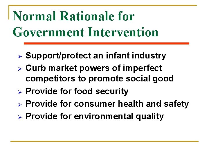
Normal Rationale for Government Intervention Ø Ø Ø Support/protect an infant industry Curb market powers of imperfect competitors to promote social good Provide for food security Provide for consumer health and safety Provide for environmental quality

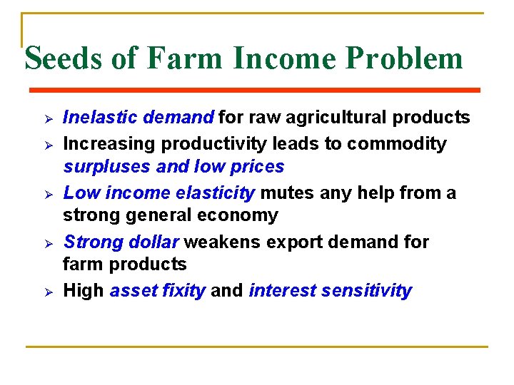
Seeds of Farm Income Problem Ø Ø Ø Inelastic demand for raw agricultural products Increasing productivity leads to commodity surpluses and low prices Low income elasticity mutes any help from a strong general economy Strong dollar weakens export demand for farm products High asset fixity and interest sensitivity

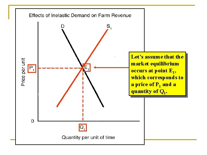
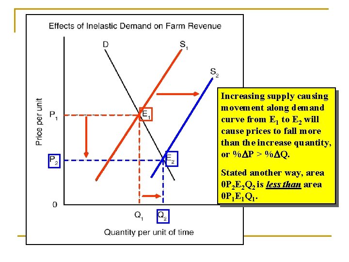
Let’s assume that the market equilibrium occurs at point E 1, which corresponds to a price of P 1 and a quantity of Q 1.

Increasing supply causing movement along demand curve from E 1 to E 2 will cause prices to fall more than the increase quantity, or % P > % Q. Stated another way, area 0 P 2 E 2 Q 2 is less than area 0 P 1 E 1 Q 1.

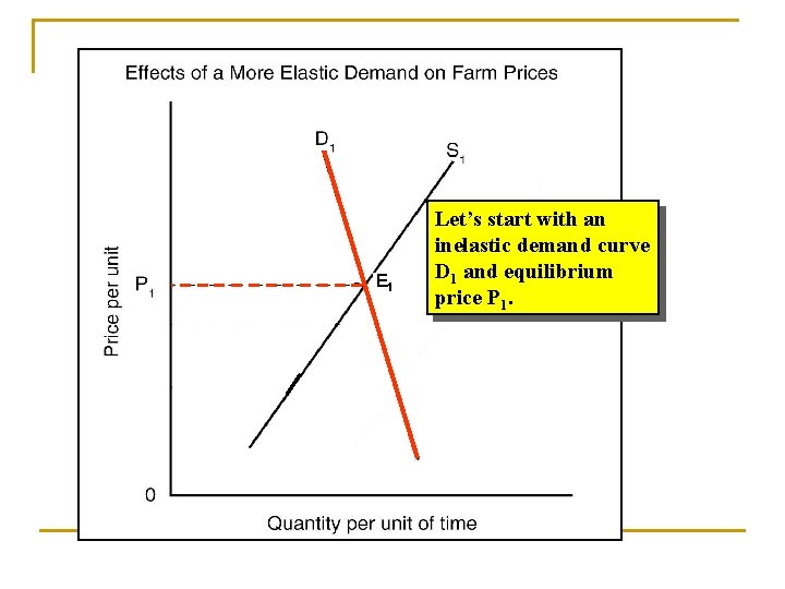
E 1 Let’s start with an inelastic demand curve D 1 and equilibrium price P 1.

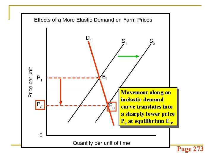
E 1 Movement along an inelastic demand curve translates into a sharply lower price P 3 at equilibrium E 3. Page 273

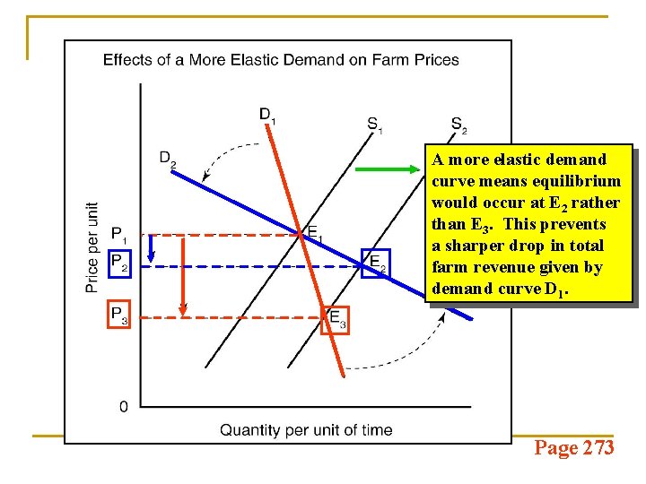
A more elastic demand curve means equilibrium would occur at E 2 rather than E 3. This prevents a sharper drop in total farm revenue given by demand curve D 1. Page 273

Forms of Government Intervention Adjusting production to market demand Ø Price and income support payments Ø Foreign trade enhancements Ø Crop insurance Ø Subsidized credit Ø Other forms Ø

Consumer Issues Adequate and cheap food supply Ø Nutrition and health issues Ø Food subsidy issues Ø Rural community issues Ø

Resource Issues Soil erosion and land use issues Ø Adequacy of water supply issues Ø Hired farm labor issues Ø Energy issues Ø

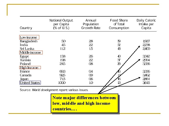
International Issues Ø Adequacy of world food supply

Note major differences between low, middle and high income countries….

International Issues Adequacy of world food supply Ø Movement towards free trade Ø

Price and Income Support A Historical perspective Ø Ø Commodity acquisition-loan rate mechanism Set-aside mechanism Target price mechanism Commodities covered by government programs

The Loan Rate Approach to Supporting Farm Prices and Income

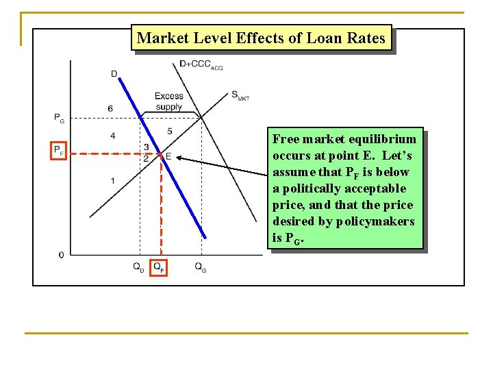
Market Level Effects of Loan Rates Free market equilibrium occurs at point E. Let’s assume that PF is below a politically acceptable price, and that the price desired by policymakers is PG.

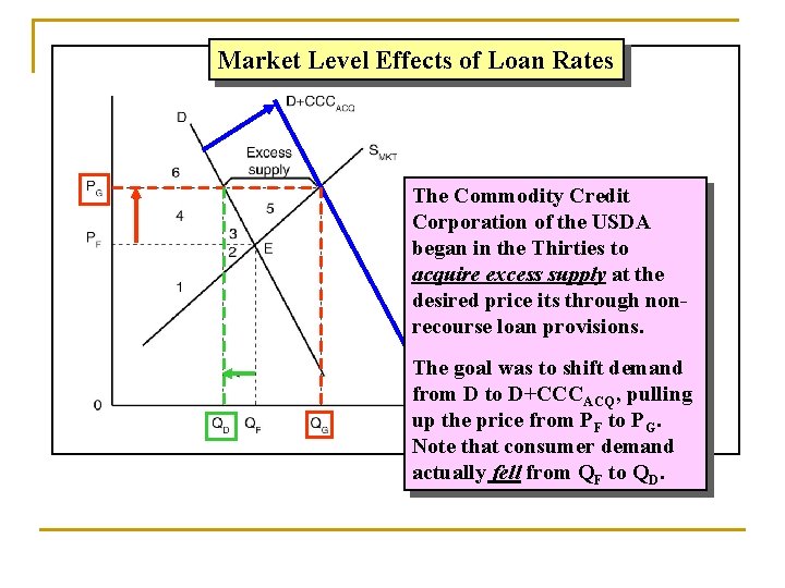
Market Level Effects of Loan Rates The Commodity Credit Corporation of the USDA began in the Thirties to acquire excess supply at the desired price its through nonrecourse loan provisions. The goal was to shift demand from D to D+CCCACQ, pulling up the price from PF to PG. Note that consumer demand actually fell from QF to QD.

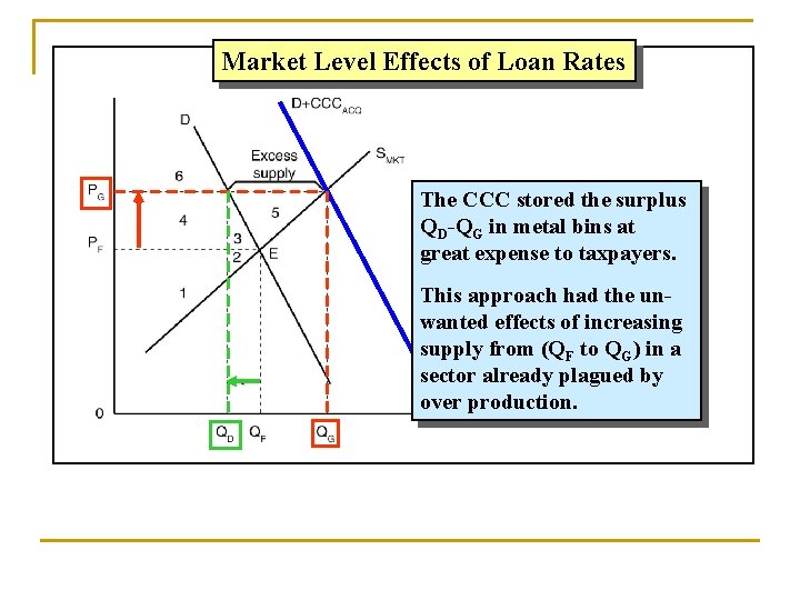
Market Level Effects of Loan Rates The CCC stored the surplus QD-QG in metal bins at great expense to taxpayers. This approach had the unwanted effects of increasing supply from (QF to QG) in a sector already plagued by over production.

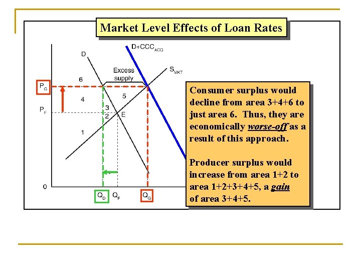
Market Level Effects of Loan Rates Consumer surplus would decline from area 3+4+6 to just area 6. Thus, they are economically worse-off as a result of this approach. Producer surplus would increase from area 1+2 to area 1+2+3+4+5, a gain of area 3+4+5.

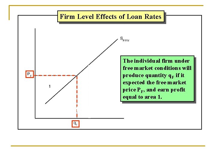
Firm Level Effects of Loan Rates The individual firm under free market conditions will produce quantity q. F if it expected the free market price PF, and earn profit equal to area 1.

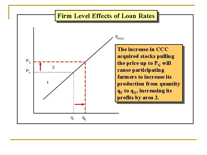
Firm Level Effects of Loan Rates The increase in CCC acquired stocks pulling the price up to PG will cause participating farmers to increase its production from quantity q. F to q. G, increasing its profits by area 2.

The Set-Aside Approach to Supporting Farm Prices and Income

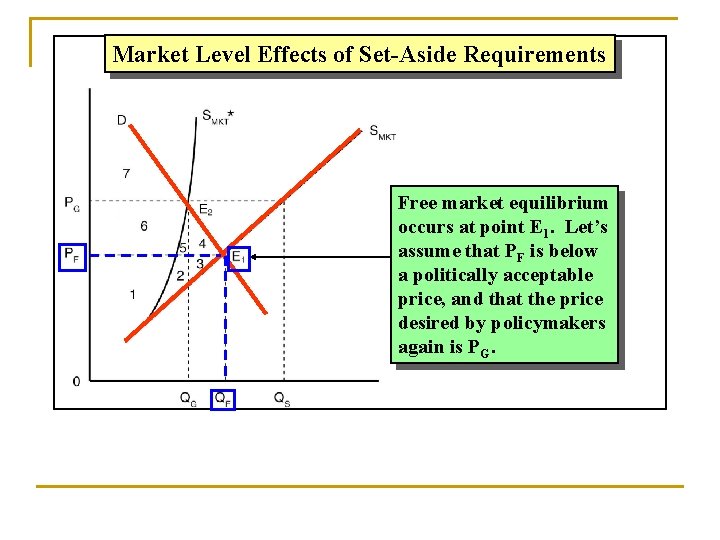
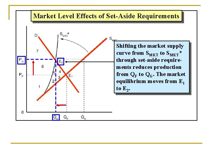
Market Level Effects of Set-Aside Requirements Free market equilibrium occurs at point E 1. Let’s assume that PF is below a politically acceptable price, and that the price desired by policymakers again is PG.

Market Level Effects of Set-Aside Requirements Shifting the market supply curve from SMKT to SMKT* through set-aside requirements reduces production from QF to QG. The market equilibrium moves from E 1 to E 2.

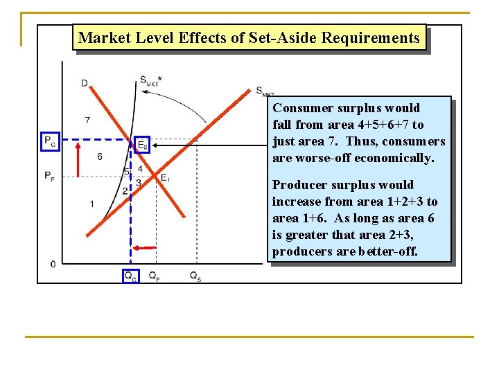
Market Level Effects of Set-Aside Requirements Consumer surplus would fall from area 4+5+6+7 to just area 7. Thus, consumers are worse-off economically. Producer surplus would increase from area 1+2+3 to area 1+6. As long as area 6 is greater that area 2+3, producers are better-off.

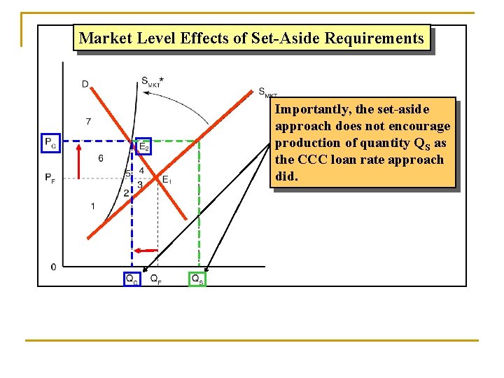
Market Level Effects of Set-Aside Requirements Importantly, the set-aside approach does not encourage production of quantity QS as the CCC loan rate approach did.

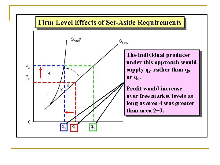
Firm Level Effects of Set-Aside Requirements The individual producer under this approach would supply q. G rather than q. F or q. S. Profit would increase over free market levels as long as area 4 was greater than area 2+3.

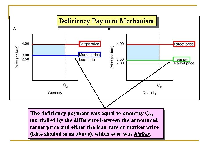
Deficiency Payment Mechanism The deficiency payment was equal to qnantity QM multiplied by the difference between the announced target price and either the loan rate or market price (blue shaded area above), which ever was higher.

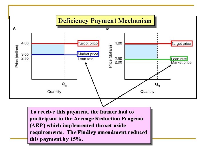
Deficiency Payment Mechanism To receive this payment, the farmer had to participant in the Acreage Reduction Program (ARP) which implemented the set-aside requirements. The Findley amendment reduced this payment by 15%.

The Current Approach to Supporting Farm Prices and Income

Some Demand Side Options

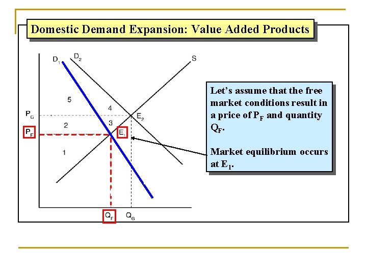
Domestic Demand Expansion: Value Added Products Let’s assume that the free market conditions result in a price of PF and quantity QF. Market equilibrium occurs at E 1.

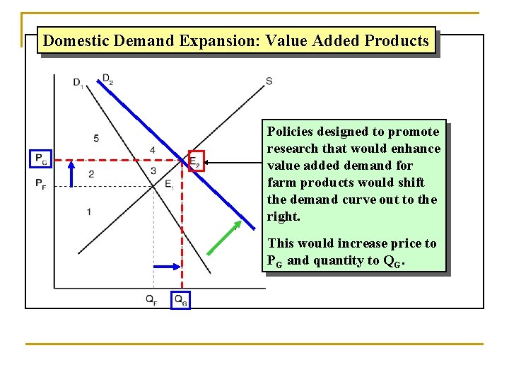
Domestic Demand Expansion: Value Added Products Policies designed to promote research that would enhance value added demand for farm products would shift the demand curve out to the right. This would increase price to PG and quantity to QG.

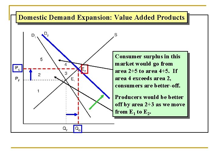
Domestic Demand Expansion: Value Added Products Consumer surplus in this market would go from area 2+5 to area 4+5. If area 4 exceeds area 2, consumers are better-off. Producers would be better off by area 2+3 as we move from E 1 to E 2.

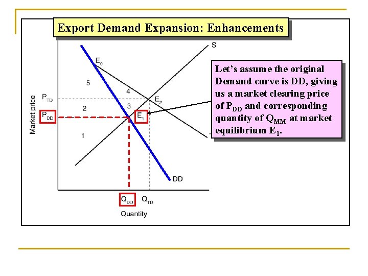
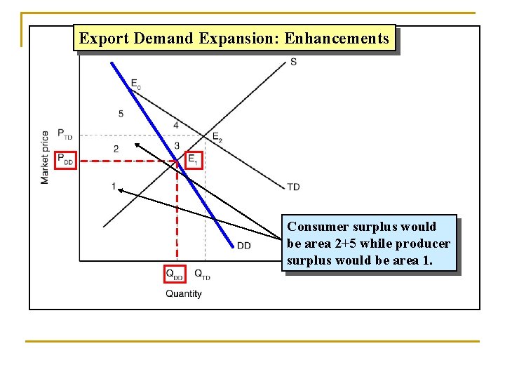
Export Demand Expansion: Enhancements Let’s assume the original Demand curve is DD, giving us a market clearing price of PDD and corresponding quantity of QMM at market equilibrium E 1.

Export Demand Expansion: Enhancements Consumer surplus would be area 2+5 while producer surplus would be area 1.

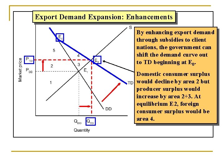
Export Demand Expansion: Enhancements By enhancing export demand through subsidies to client nations, the government can shift the demand curve out to TD beginning at E 0. Domestic consumer surplus would decline by area 2 but producer surplus would increase by area 2+3. At equilibrium E 2, foreign consumer surplus would be area 4.

Agricultural Support Policies in Turkey

Price Supports n n n Commodity loans for wheat Commodity loans for tobacco Commodity loans for sugar

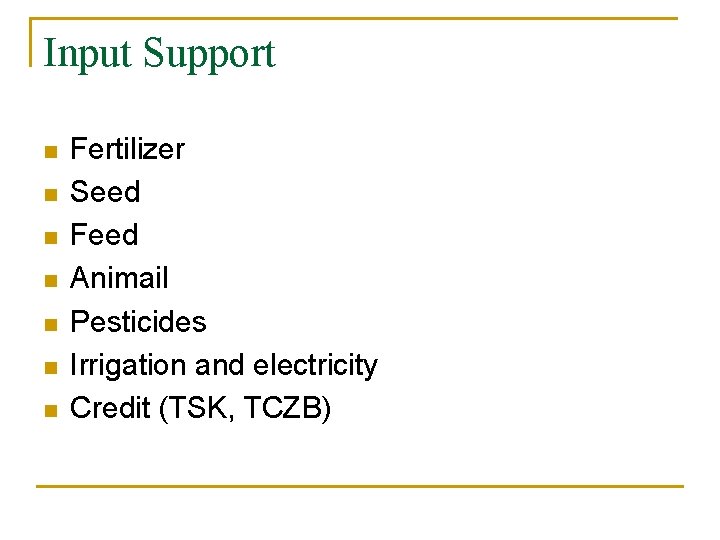
Input Support n n n n Fertilizer Seed Feed Animail Pesticides Irrigation and electricity Credit (TSK, TCZB)

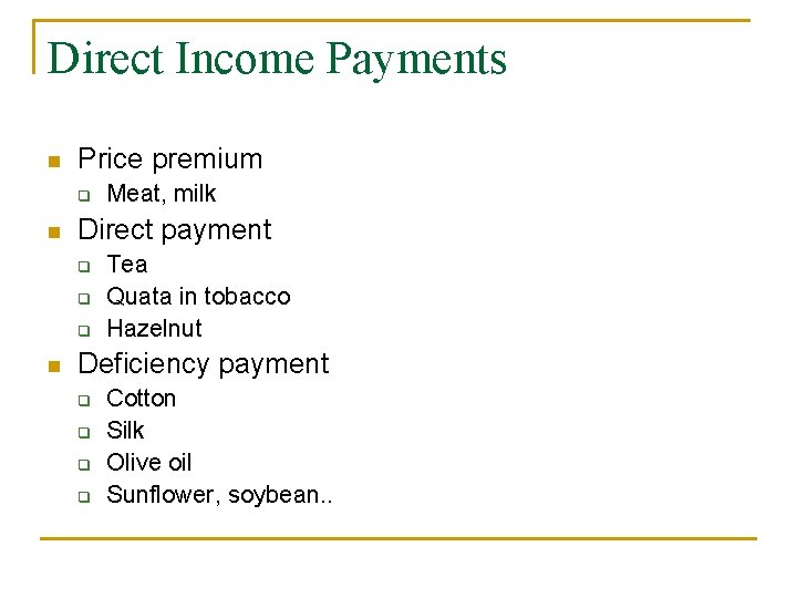
Direct Income Payments n Price premium q n Direct payment q q q n Meat, milk Tea Quata in tobacco Hazelnut Deficiency payment q q Cotton Silk Olive oil Sunflower, soybean. .