Agricultural Economics Lecture 2 Foundations of Microeconomics in

Agricultural Economics Lecture 2: Foundations of Microeconomics in Agriculture Powerpoint tranparencies from Penson, et. al. 3 rd. Ed.

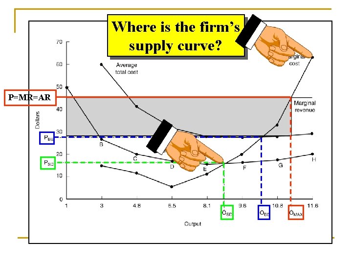
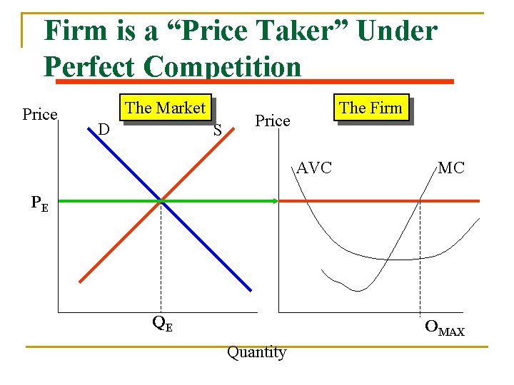
Where is the firm’s supply curve? P=MR=AR

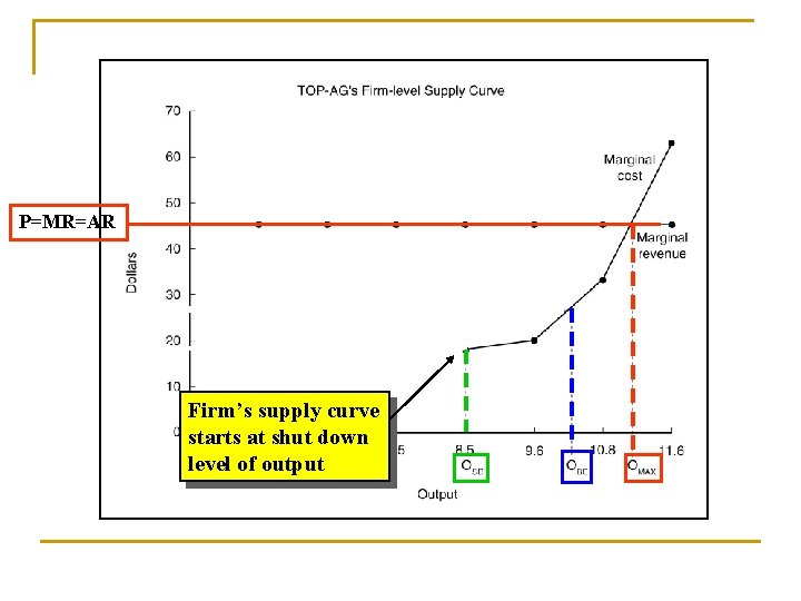
P=MR=AR Firm’s supply curve starts at shut down level of output

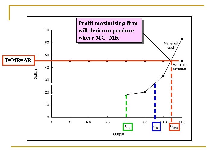
Profit maximizing firm will desire to produce where MC=MR P=MR=AR

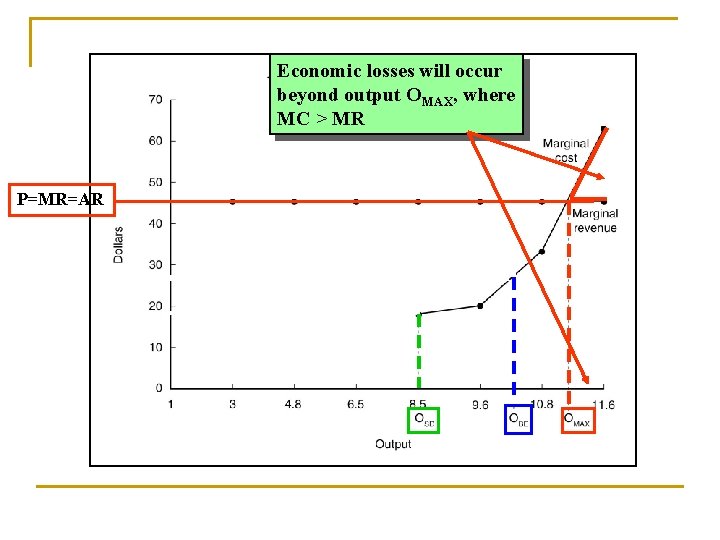
Economic losses will occur beyond output OMAX, where MC > MR P=MR=AR

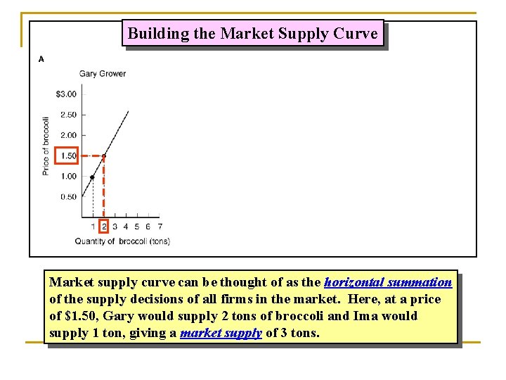
Building the Market Supply Curve Market supply curve can be thought of as the horizontal summation of the supply decisions of all firms in the market. Here, at a price of $1. 50, Gary would supply 2 tons of broccoli and Ima would supply 1 ton, giving a market supply of 3 tons.

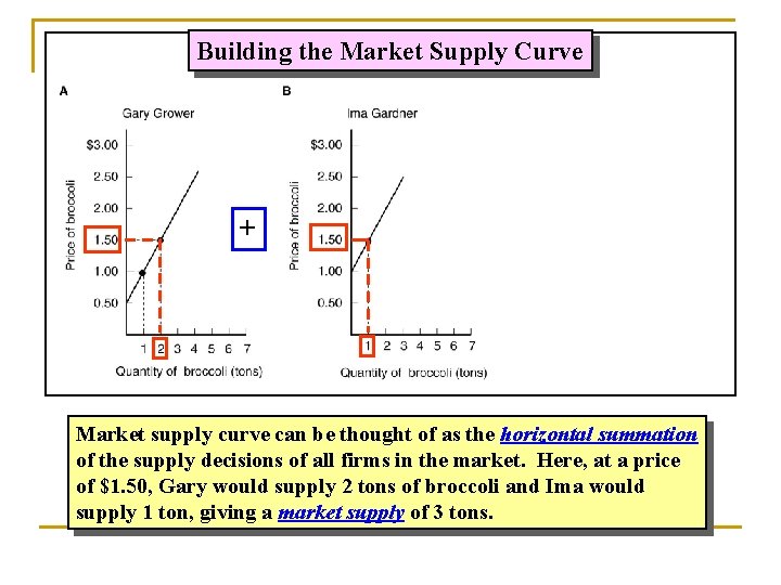
Building the Market Supply Curve + Market supply curve can be thought of as the horizontal summation of the supply decisions of all firms in the market. Here, at a price of $1. 50, Gary would supply 2 tons of broccoli and Ima would supply 1 ton, giving a market supply of 3 tons.

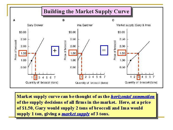
Building the Market Supply Curve + = Market supply curve can be thought of as the horizontal summation of the supply decisions of all firms in the market. Here, at a price of $1. 50, Gary would supply 2 tons of broccoli and Ima would supply 1 ton, giving a market supply of 3 tons.

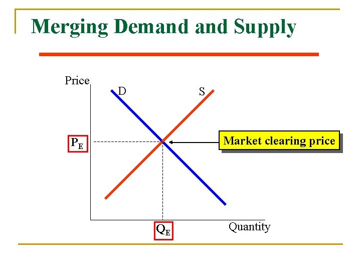
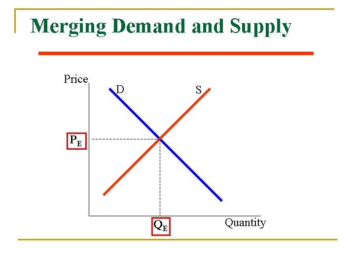
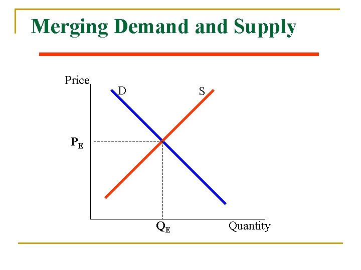
Merging Demand Supply Price D S Market clearing price PE QE Quantity

Merging Demand Supply Price D S PE QE Quantity

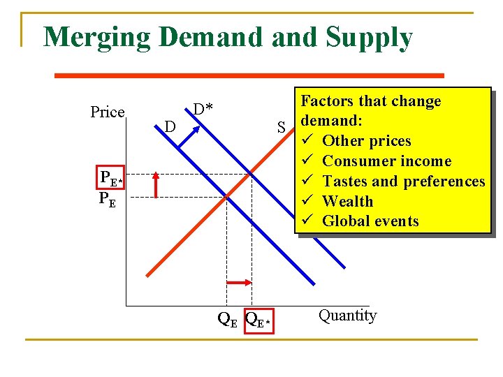
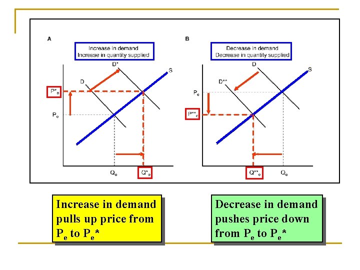
Merging Demand Supply Price D Factors that change S demand: ü Other prices ü Consumer income ü Tastes and preferences ü Wealth ü Global events D* PE QE QE* Quantity

Merging Demand Supply Price D S PE QE Quantity

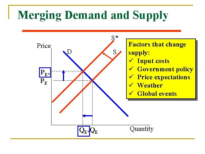
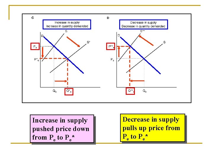
Merging Demand Supply S* Price D S PE* PE QE*QE Factors that change supply: ü Input costs ü Government policy ü Price expectations ü Weather ü Global events Quantity

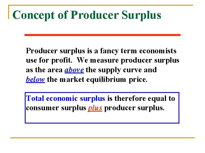
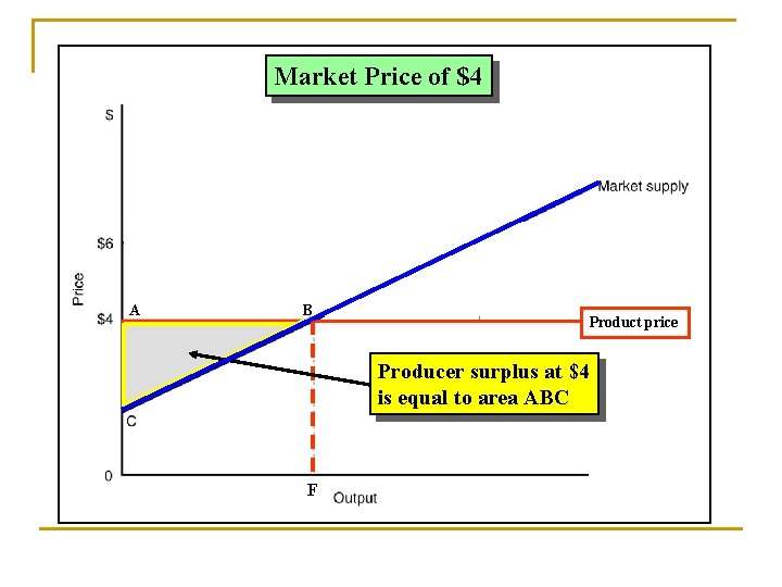
Concept of Producer Surplus Producer surplus is a fancy term economists use for profit. We measure producer surplus as the area above the supply curve and below the market equilibrium price.

Concept of Producer Surplus Producer surplus is a fancy term economists use for profit. We measure producer surplus as the area above the supply curve and below the market equilibrium price. Total economic surplus is therefore equal to consumer surplus producer surplus.

Market Price of $4 A B Product price Producer surplus at $4 is equal to area ABC F G

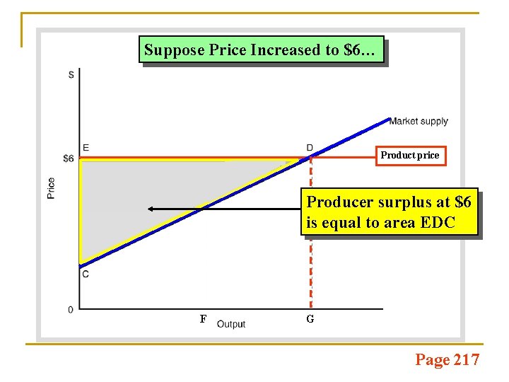
Suppose Price Increased to $6… Product price Producer surplus at $6 is equal to area EDC F G Page 217

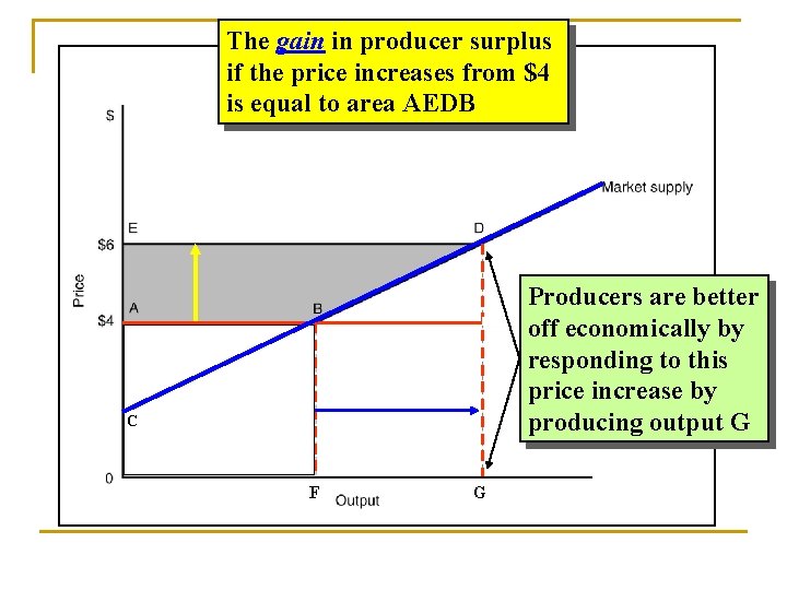
The gain in producer surplus if the price increases from $4 is equal to area AEDB Producers are better off economically by responding to this price increase by producing output G C F G

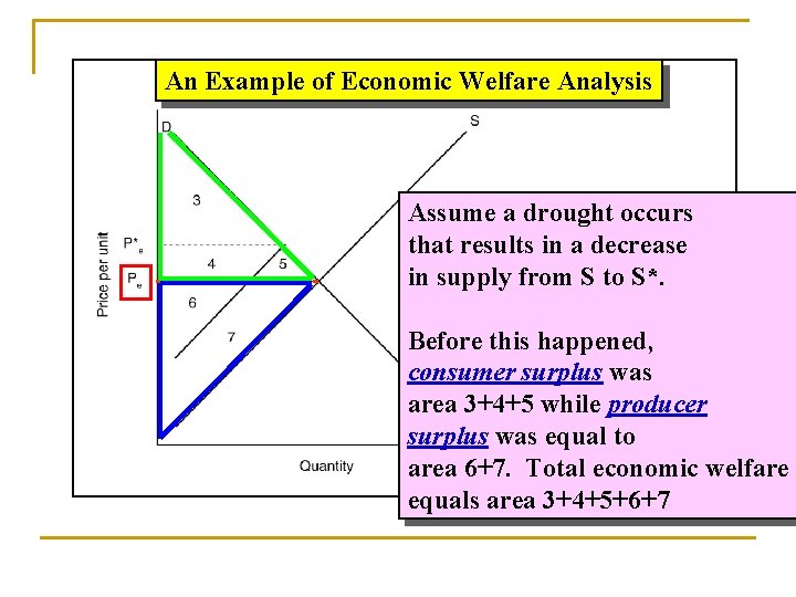
An Example of Economic Welfare Analysis Assume a drought occurs that results in a decrease in supply from S to S*. Before this happened, consumer surplus was area 3+4+5 while producer surplus was equal to area 6+7. Total economic welfare equals area 3+4+5+6+7

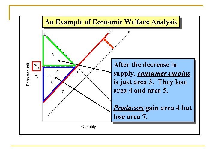
An Example of Economic Welfare Analysis After the decrease in supply, consumer surplus is just area 3. They lose area 4 and area 5. Producers gain area 4 but lose area 7.

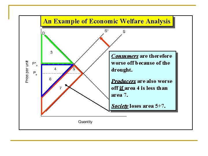
An Example of Economic Welfare Analysis Consumers are therefore worse off because of the drought. Producers are also worse off if area 4 is less than area 7. Society loses area 5+7.

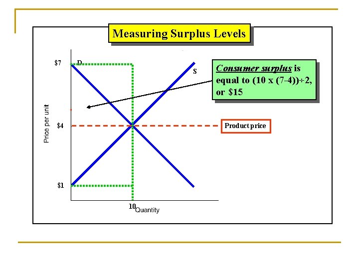
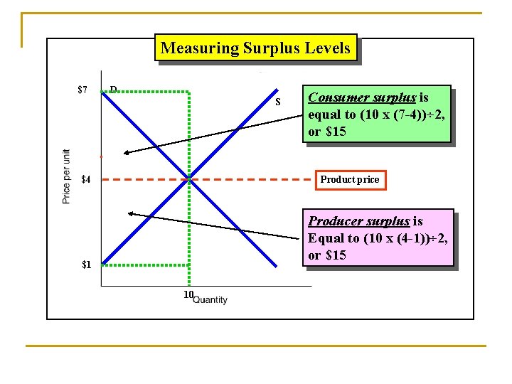
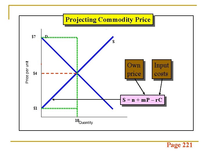
Measuring Surplus Levels $7 D S $4 Consumer surplus is equal to (10 x (7 -4))÷ 2, or $15 Product price $1 10

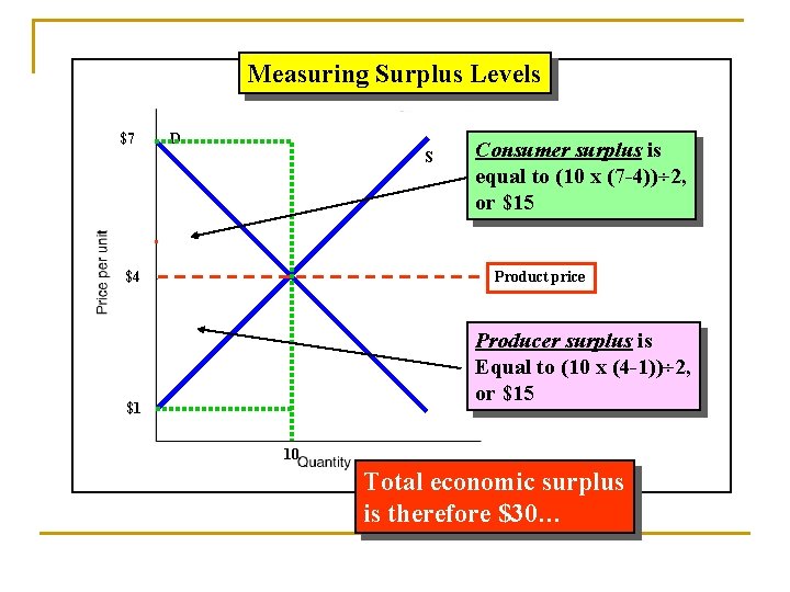
Measuring Surplus Levels $7 D S $4 Consumer surplus is equal to (10 x (7 -4))÷ 2, or $15 Product price Producer surplus is Equal to (10 x (4 -1))÷ 2, or $15 $1 10

Measuring Surplus Levels $7 D S $4 Consumer surplus is equal to (10 x (7 -4))÷ 2, or $15 Product price Producer surplus is Equal to (10 x (4 -1))÷ 2, or $15 $1 10 Total economic surplus is therefore $30…

Modeling Commodity Prices

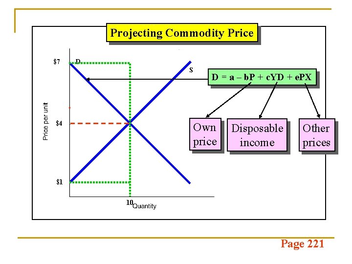
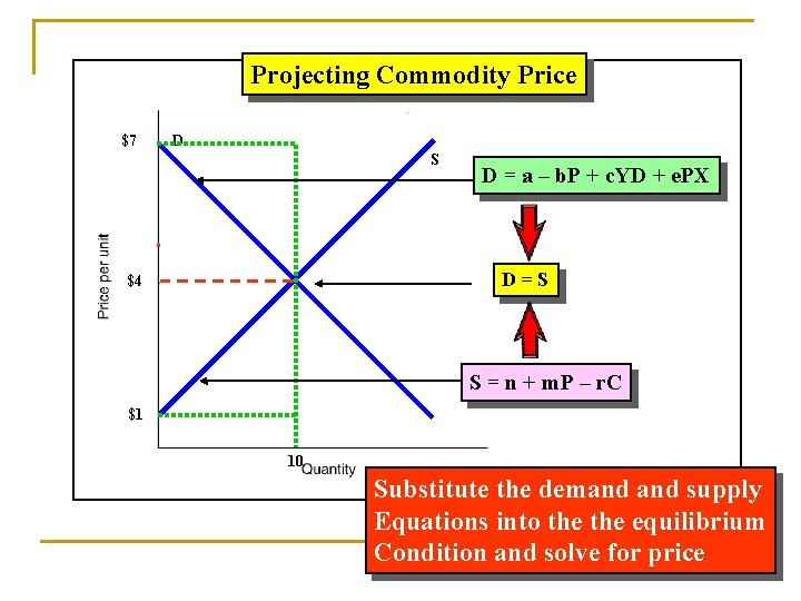
Projecting Commodity Price $7 D S $4 D = a – b. P + c. YD + e. PX Own price Disposable income Other prices $1 10 Page 221

Projecting Commodity Price $7 D S Own price $4 Input costs S = n + m. P – r. C $1 10 Page 221

Projecting Commodity Price $7 D S D = a – b. P + c. YD + e. PX D=S $4 S = n + m. P – r. C $1 10 Substitute the demand supply Equations into the equilibrium Condition and solve for. Page price 221

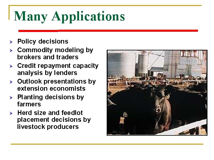
Many Applications Ø Ø Ø Policy decisions Commodity modeling by brokers and traders Credit repayment capacity analysis by lenders Outlook presentations by extension economists Planting decisions by farmers Herd size and feedlot placement decisions by livestock producers

Market Disequilibrium

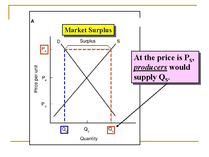
Market Surplus At the price is PS, producers would supply QS.

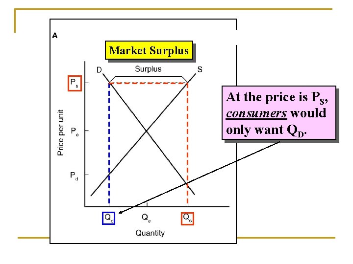
Market Surplus At the price is PS, consumers would only want QD.

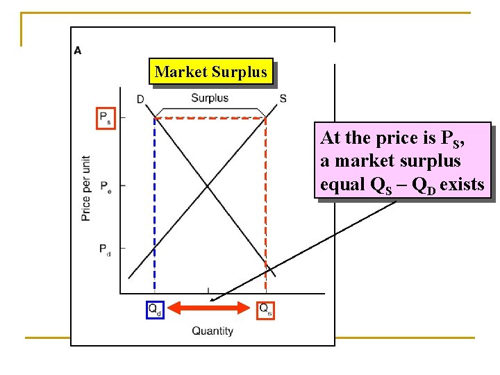
Market Surplus At the price is PS, a market surplus equal QS – QD exists

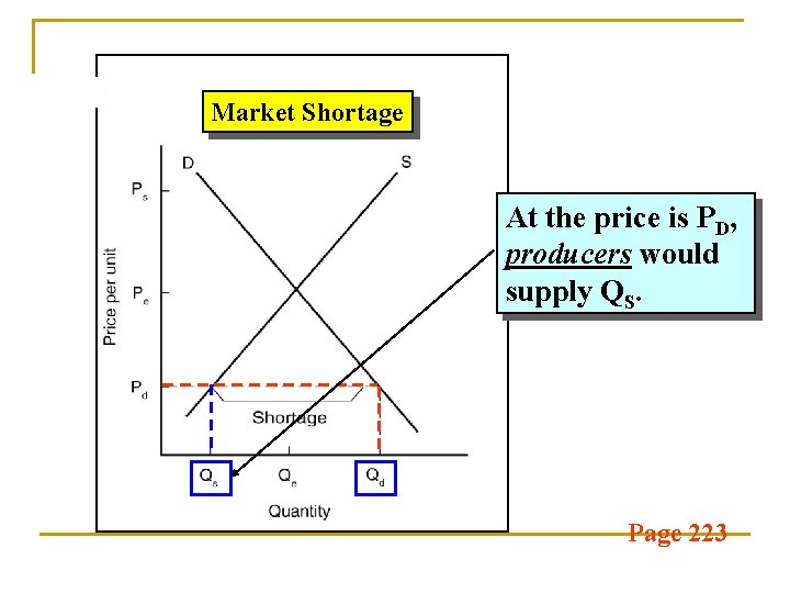
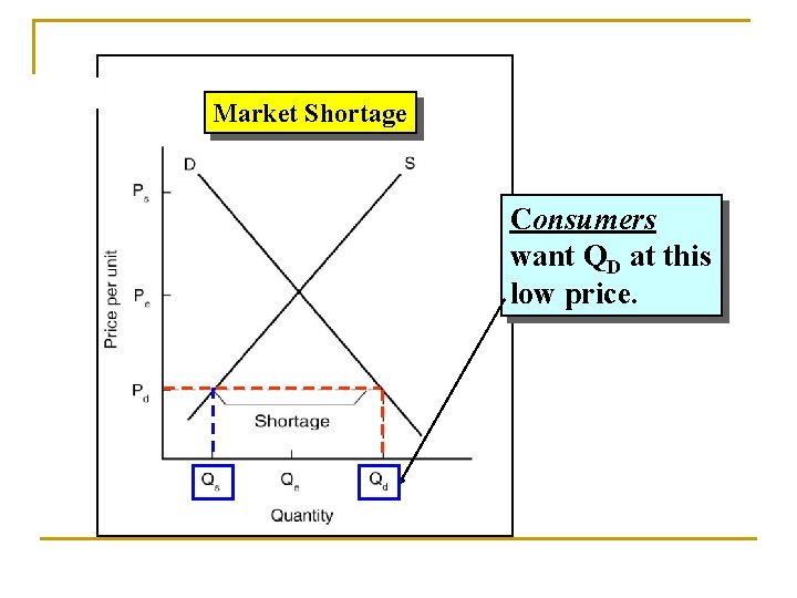
Market Shortage At the price is PD, producers would supply QS. Page 223

Market Shortage Consumers want QD at this low price.

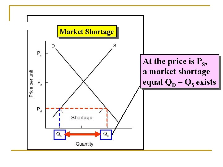
Market Shortage At the price is PS, Consumers awant market QD at shortage this low price. equal QD – QS exists

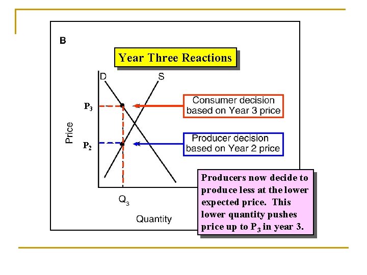
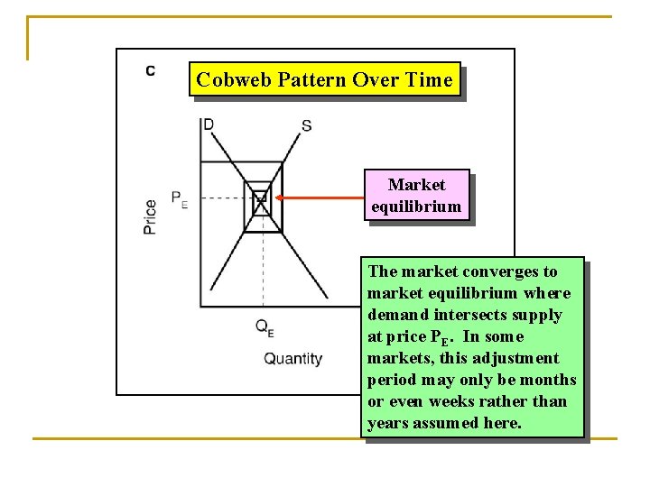
Adjustments to Market Equilibrium Markets converge to equilibrium over time unless other events in the economy occur. One explanation for this adjustment which makes sense in agriculture is the Cobweb theory. This names stems from the spider like trail the adjustment process makes.

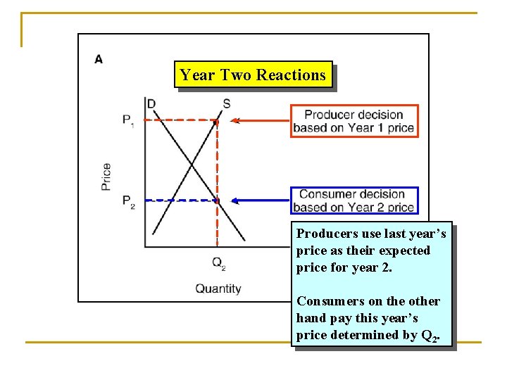
Year Two Reactions Producers use last year’s price as their expected price for year 2. Consumers on the other hand pay this year’s price determined by Q 2.

Year Three Reactions P 3 P 2 Producers now decide to produce less at the lower expected price. This lower quantity pushes price up to P 3 in year 3.

Cobweb Pattern Over Time Market equilibrium The market converges to market equilibrium where demand intersects supply at price PE. In some markets, this adjustment period may only be months or even weeks rather than years assumed here.

Market-to-Firm Linkages

Some Important Jargon We need to distinguish between movement along a demand or supply curve, and shifts in the demand or supply curve.

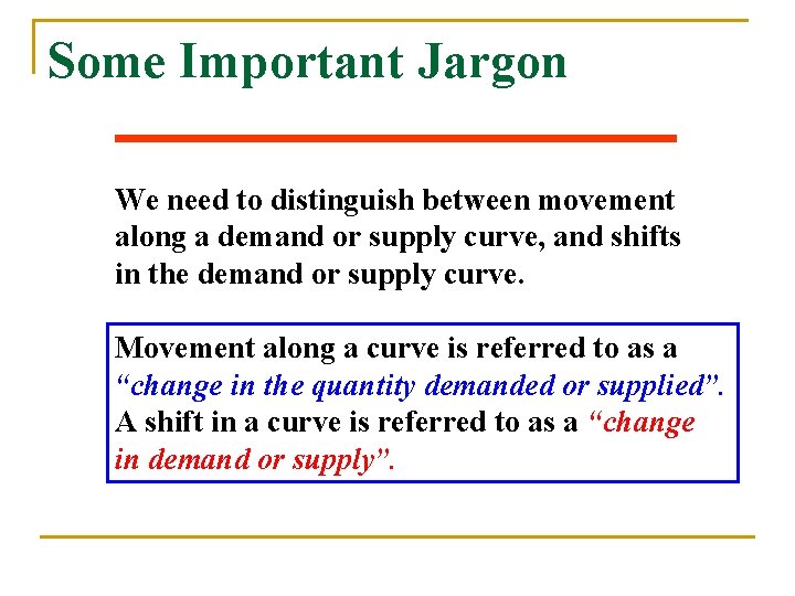
Some Important Jargon We need to distinguish between movement along a demand or supply curve, and shifts in the demand or supply curve. Movement along a curve is referred to as a “change in the quantity demanded or supplied”. A shift in a curve is referred to as a “change in demand or supply”.

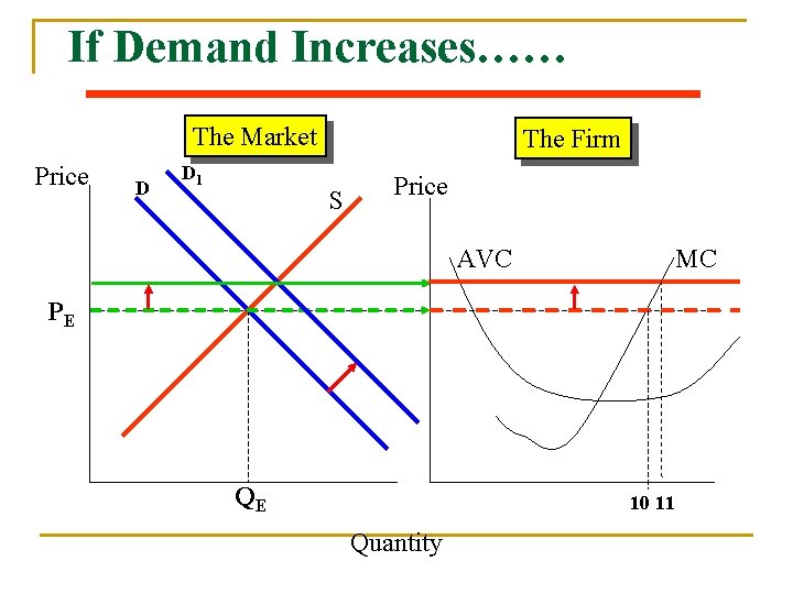
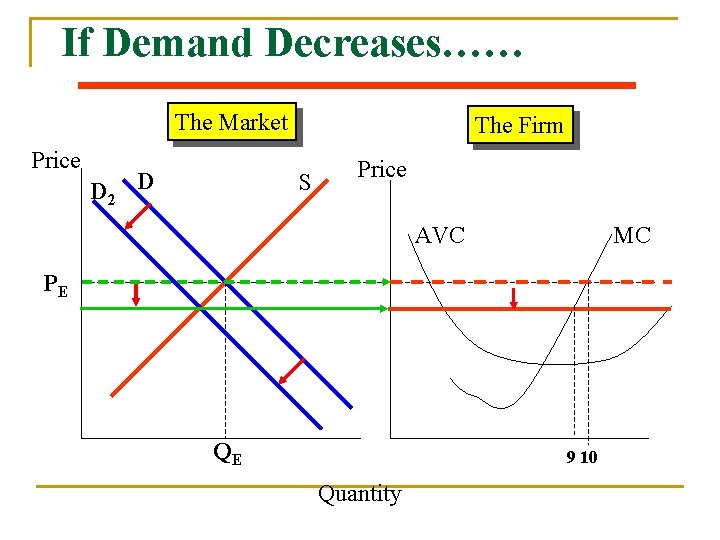
Increase in demand pulls up price from Pe to Pe* Decrease in demand pushes price down from Pe to Pe*

Increase in supply pushed price down from Pe to Pe* Decrease in supply pulls up price from Pe to Pe*

Merging Demand Supply Price D S PE QE Quantity

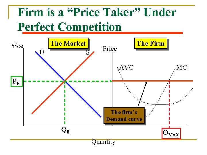
Firm is a “Price Taker” Under Perfect Competition Price The Market D S The Firm Price AVC MC PE QE OMAX Quantity

If Demand Increases…… The Market Price D D 1 The Firm S Price AVC MC PE QE 10 11 Quantity

If Demand Decreases…… The Market Price D 2 D The Firm S Price AVC MC PE QE 9 10 Quantity

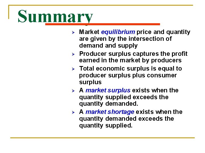
Summary Ø Ø Ø Market equilibrium price and quantity are given by the intersection of demand supply Producer surplus captures the profit earned in the market by producers Total economic surplus is equal to producer surplus consumer surplus A market surplus exists when the quantity supplied exceeds the quantity demanded. A market shortage exists when the quantity demanded exceeds the quantity supplied.

Market Equilibrium and Market Demand: Imperfect Competition

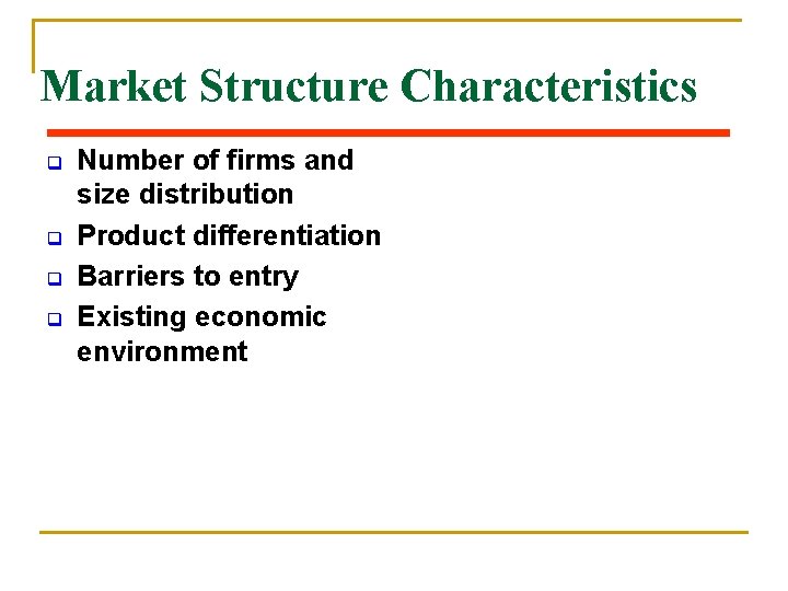
Market Structure Characteristics q q Number of firms and size distribution Product differentiation Barriers to entry Existing economic environment

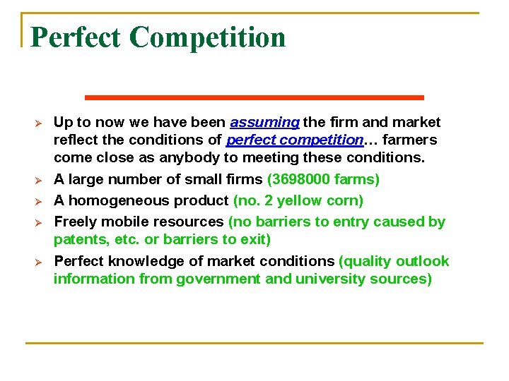
Perfect Competition Ø Ø Ø Up to now we have been assuming the firm and market reflect the conditions of perfect competition… farmers come close as anybody to meeting these conditions. A large number of small firms (3698000 farms) A homogeneous product (no. 2 yellow corn) Freely mobile resources (no barriers to entry caused by patents, etc. or barriers to exit) Perfect knowledge of market conditions (quality outlook information from government and university sources)

Firm is a “Price Taker” Under Perfect Competition Price The Market D S The Firm Price AVC MC PE The firm’s Demand curve QE OMAX Quantity

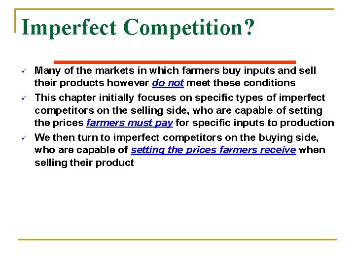
Imperfect Competition? ü ü ü Many of the markets in which farmers buy inputs and sell their products however do not meet these conditions This chapter initially focuses on specific types of imperfect competitors on the selling side, who are capable of setting the prices farmers must pay for specific inputs to production We then turn to imperfect competitors on the buying side, who are capable of setting the prices farmers receive when selling their product

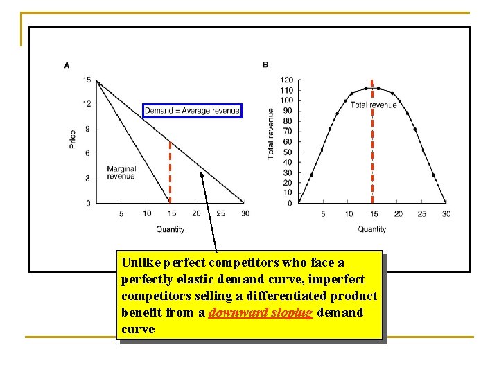
Unlike perfect competitors who face a perfectly elastic demand curve, imperfect competitors selling a differentiated product benefit from a downward sloping demand curve

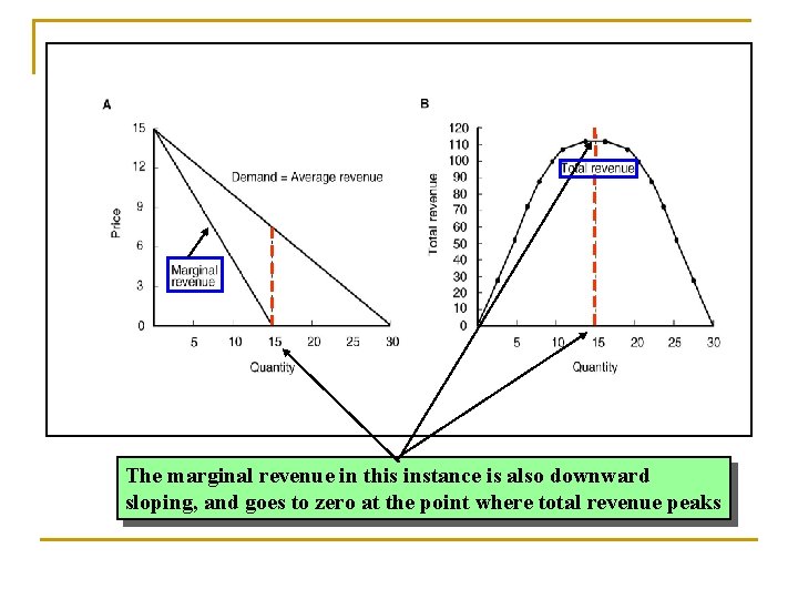
The marginal revenue in this instance is also downward sloping, and goes to zero at the point where total revenue peaks

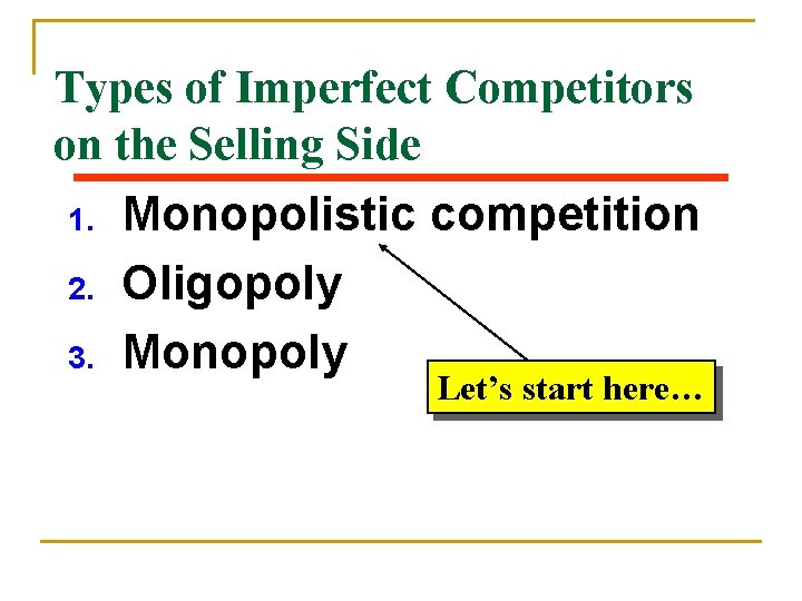
Types of Imperfect Competitors on the Selling Side 1. 2. 3. Monopolistic competition Oligopoly Monopoly Let’s start here…

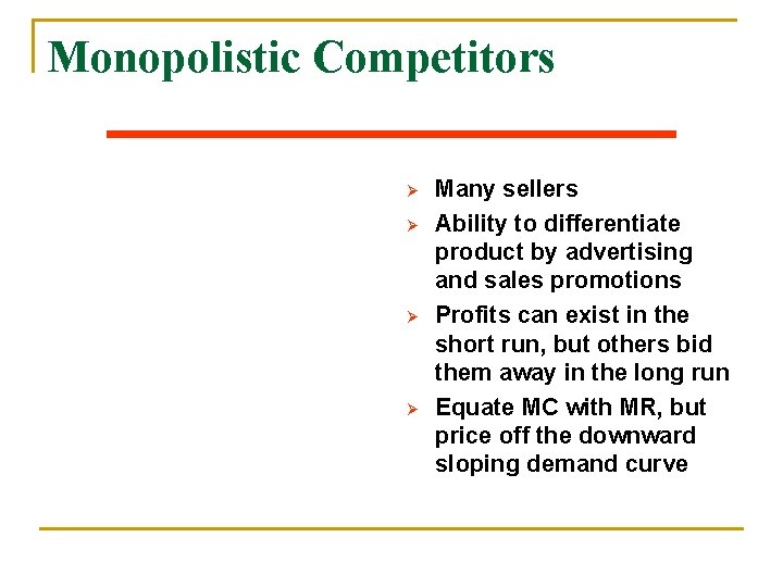
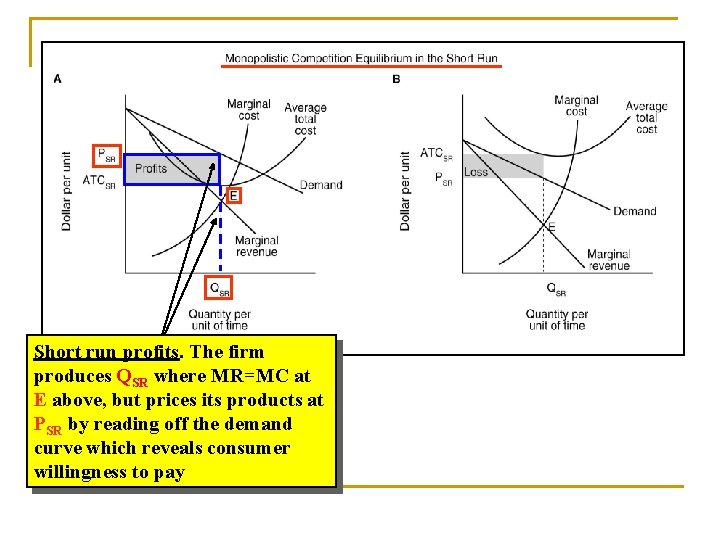
Monopolistic Competitors Ø Ø Many sellers Ability to differentiate product by advertising and sales promotions Profits can exist in the short run, but others bid them away in the long run Equate MC with MR, but price off the downward sloping demand curve

Short run profits. The firm produces QSR where MR=MC at E above, but prices its products at PSR by reading off the demand curve which reveals consumer willingness to pay

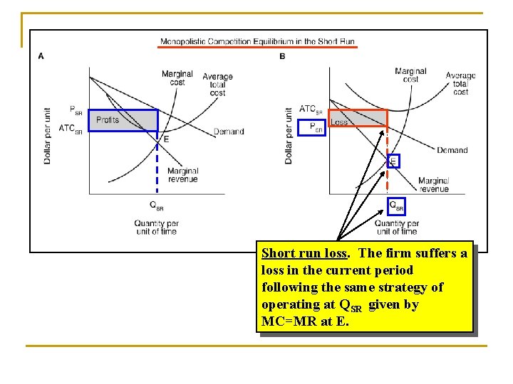
Short run loss. The firm suffers a loss in the current period following the same strategy of operating at QSR given by MC=MR at E.

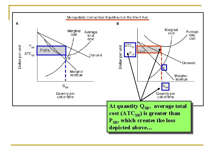
At quantity QSR, average total cost (ATCSR) is greater than PSR, which creates the loss depicted above…

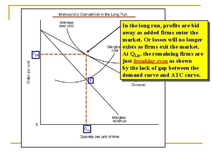
In the long run, profits are bid away as added firms enter the market. Or losses will no longer exists as firms exit the market. At QLR, the remaining firms are just breaking even as shown by the lack of gap between the demand curve and ATC curve.

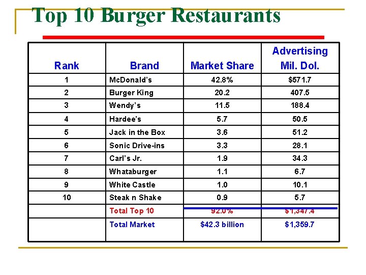
Top 10 Burger Restaurants Rank Brand Market Share Advertising Mil. Dol. 1 Mc. Donald’s 42. 8% $571. 7 2 Burger King 20. 2 407. 5 3 Wendy’s 11. 5 188. 4 4 Hardee’s 5. 7 50. 5 5 Jack in the Box 3. 6 51. 2 6 Sonic Drive-ins 3. 3 28. 1 7 Carl’s Jr. 1. 9 34. 3 8 Whataburger 1. 1 6. 7 9 White Castle 1. 0 10. 1 10 Steak n Shake 0. 9 5. 7 Total Top 10 92. 0% $1, 347. 4 Total Market $42. 3 billion $1, 359. 7

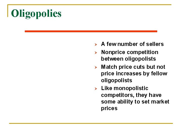
Oligopolies Ø Ø A few number of sellers Nonprice competition between oligopolists Match price cuts but not price increases by fellow oligopolists Like monopolistic competitors, they have some ability to set market prices

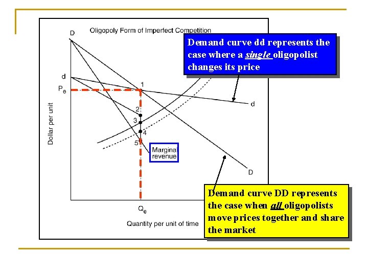
Demand curve dd represents the case where a single oligopolist changes its price Demand curve DD represents the case when all oligopolists move prices together and share the market

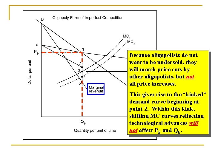
Because oligopolists do not want to be undersold, they will match price cuts by other oligopolists, but not all price increases. This gives rise to the “kinked” demand curve beginning at point 2. Within this kink, shifting MC curves reflecting technological advances will not affect PE and QE.

Monopolies Ø Ø Ø Only seller in the market Entry of other firms is restricted by patents, etc. They have absolute power over setting market price They produce a unique product They can make economic profits in the long run because they can set price without competition.

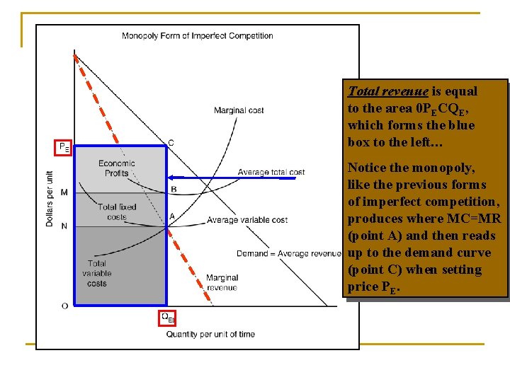
Total revenue is equal to the area 0 PECQE, which forms the blue box to the left… Notice the monopoly, like the previous forms of imperfect competition, produces where MC=MR (point A) and then reads up to the demand curve (point C) when setting price PE.

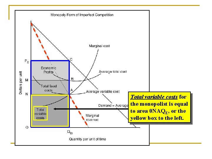
Total variable costs for the monopolist is equal to area 0 NAQE, or the yellow box to the left.

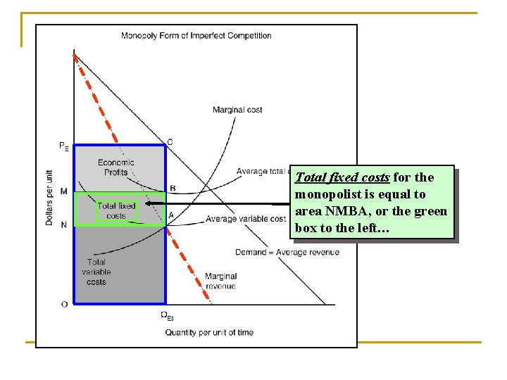
Total fixed costs for the monopolist is equal to area NMBA, or the green box to the left…

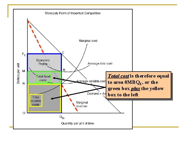
Total cost is therefore equal to area 0 MBQE, or the green box plus the yellow box to the left

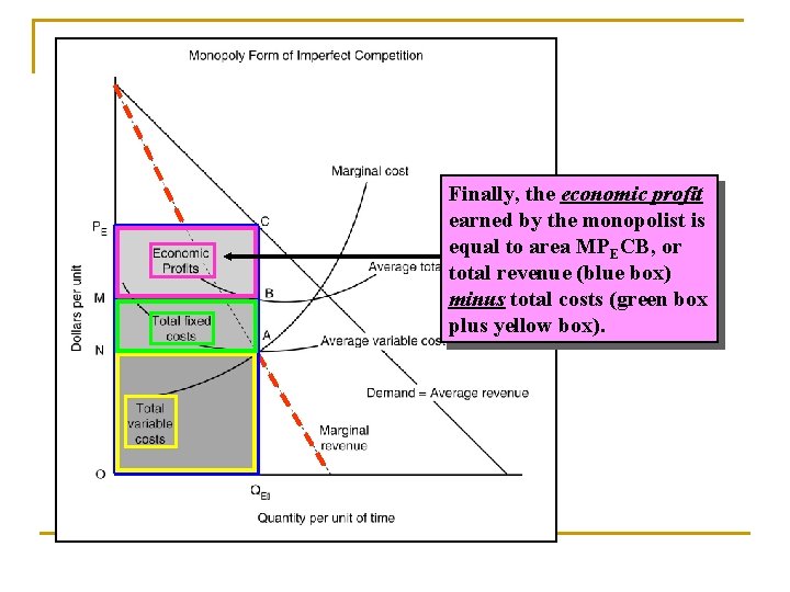
Finally, the economic profit earned by the monopolist is equal to area MPECB, or total revenue (blue box) minus total costs (green box plus yellow box).

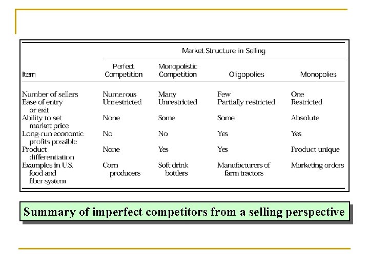
Summary of imperfect competitors from a selling perspective

Types of Imperfect Competitors on the Buying Side 1. 2. 3. Monopsonistic competition Oligopsony Let’s start here… Monopsony

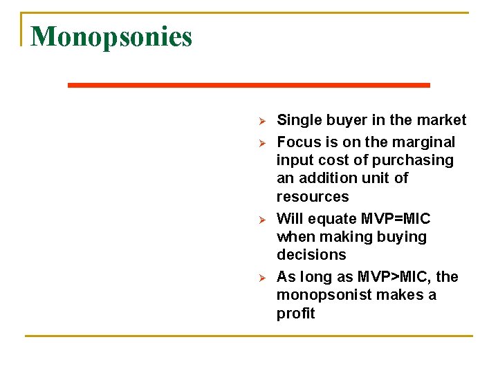
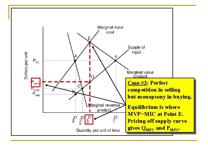
Monopsonies Ø Ø Single buyer in the market Focus is on the marginal input cost of purchasing an addition unit of resources Will equate MVP=MIC when making buying decisions As long as MVP>MIC, the monopsonist makes a profit

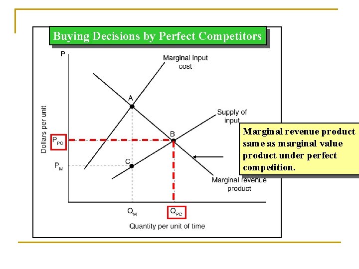
Buying Decisions by Perfect Competitors Marginal revenue product same as marginal value product under perfect competition.

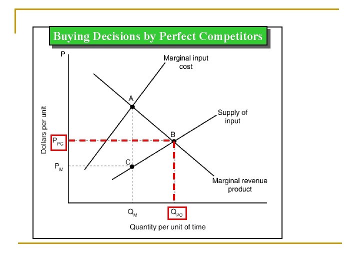
Buying Decisions by Perfect Competitors

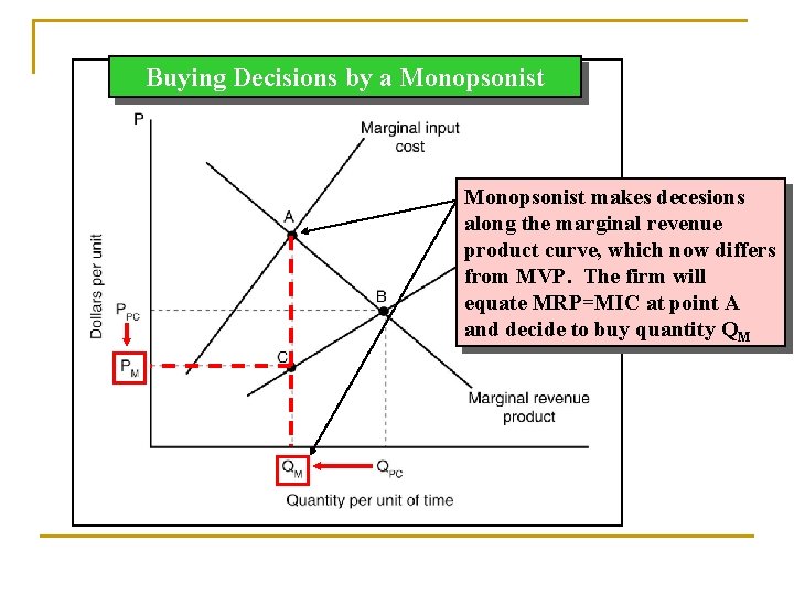
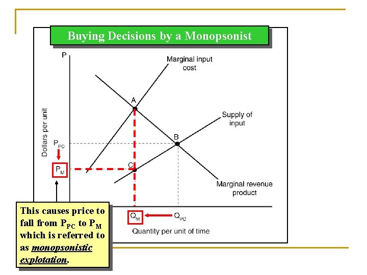
Buying Decisions by a Monopsonist makes decesions along the marginal revenue product curve, which now differs from MVP. The firm will equate MRP=MIC at point A and decide to buy quantity QM

Buying Decisions by a Monopsonist This causes price to fall from PPC to PM which is referred to as monopsonistic explotation.

Equilibrium Conditions Under Alternative Combinations of Monopsony, Monopoly, and Perfect Competition

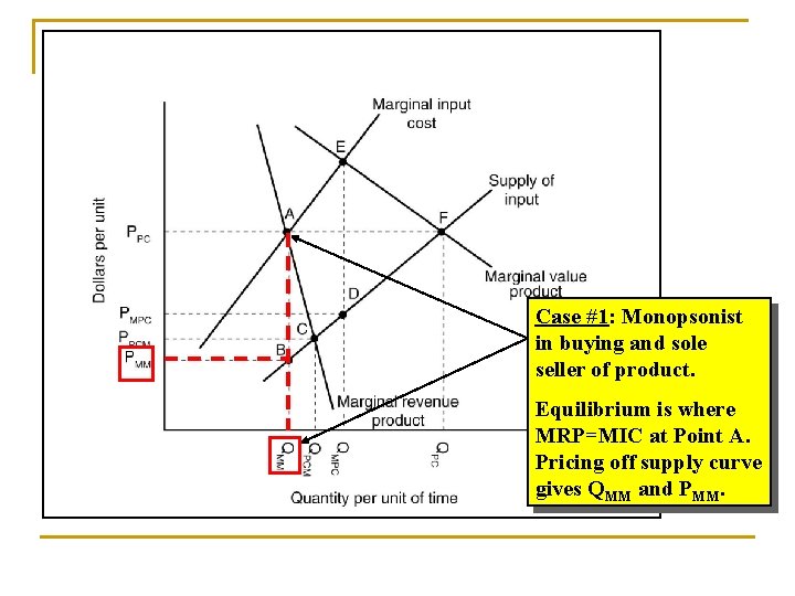
Case #1: Monopsonist in buying and sole seller of product. Equilibrium is where MRP=MIC at Point A. Pricing off supply curve gives QMM and PMM.

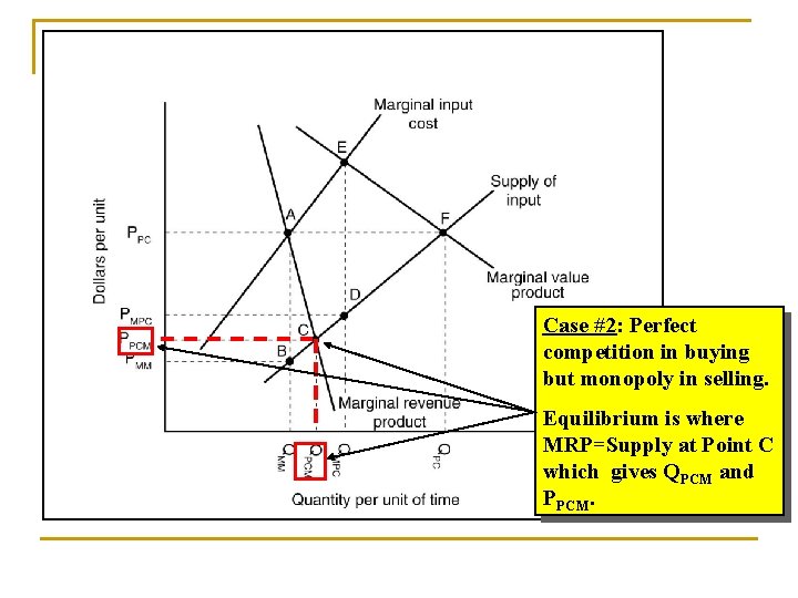
Case #2: Perfect competition in buying but monopoly in selling. Equilibrium is where MRP=Supply at Point C which gives QPCM and PPCM.

Case #3: Perfect competition in selling but monopsony in buying. Equilibrium is where MVP=MIC at Point E. Pricing off supply curve gives QMPC and PMPC.

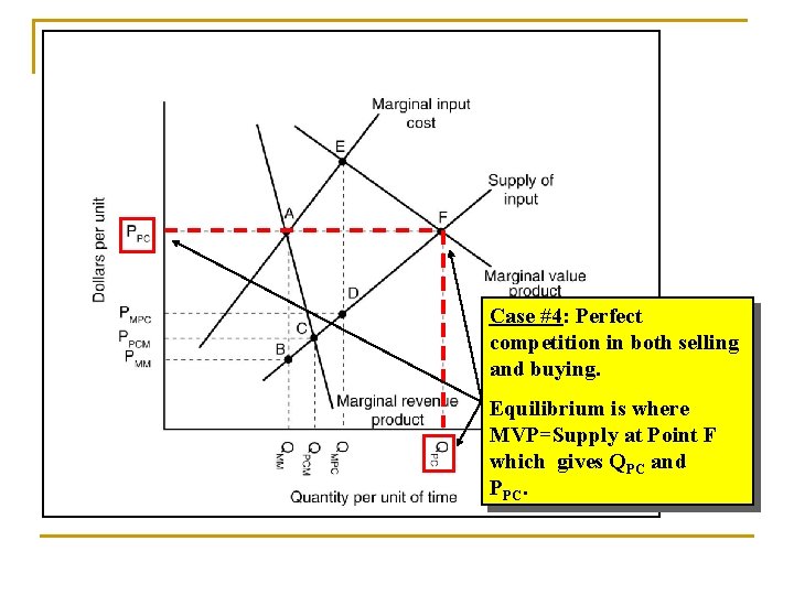
Case #4: Perfect competition in both selling and buying. Equilibrium is where MVP=Supply at Point F which gives QPC and PPC.

Monopsonistic Competitors Ø Ø Many firms buying resources Ability to differentiate services to producers Differentiated services includes distribution convenience and location of facilities, willingness to provide credit or technical assistance P and Q determined same as monopsonist

Oligopsonies Ø Ø A few number of buyers of a resource Profit earned will depend on elasticity of supply for resource (less elastic than monopsonistic competition Each oligopsonist knows fellow oligopsonists will respond to changes in price or quantity it might initiate P and Q determined same as monopsonist

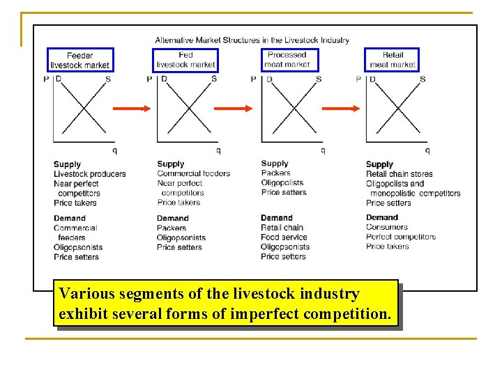
Various segments of the livestock industry exhibit several forms of imperfect competition.

Governmental Regulatory Measures Various approaches have been taken over time to counteract adverse effects of imperfect competition in the marketplace. These include: Price ceilings Lump-sum Tax Minimum price or floors

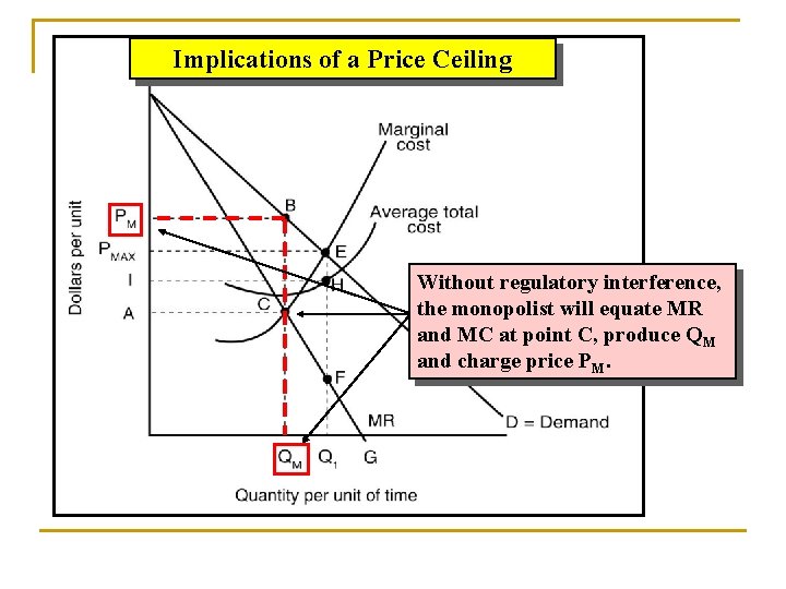
Implications of a Price Ceiling Without regulatory interference, the monopolist will equate MR and MC at point C, produce QM and charge price PM.

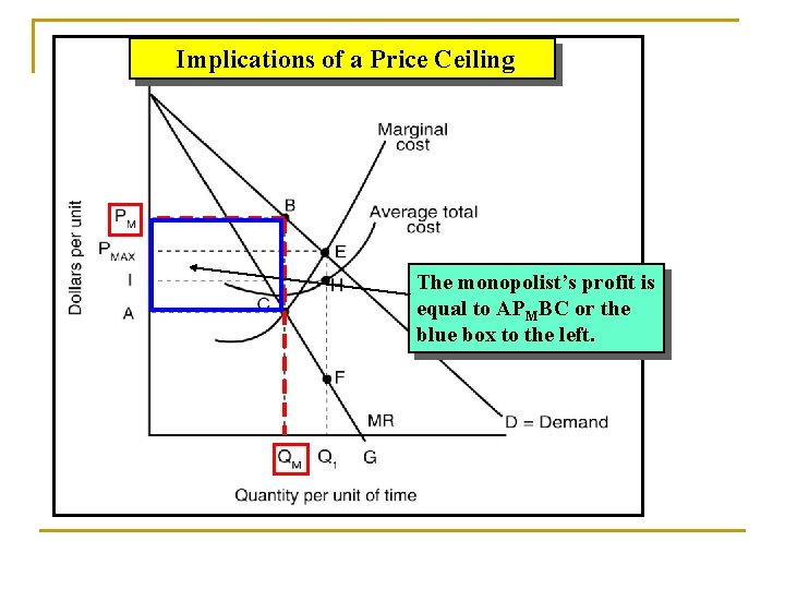
Implications of a Price Ceiling The monopolist’s profit is equal to APMBC or the blue box to the left.

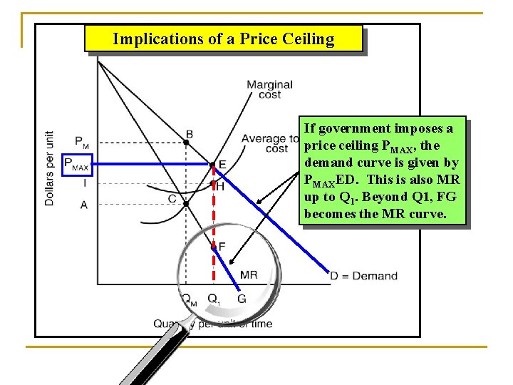
Implications of a Price Ceiling If government imposes a price ceiling PMAX, the demand curve is given by PMAXED. This is also MR up to Q 1. Beyond Q 1, FG becomes the MR curve.

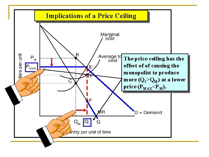
Implications of a Price Ceiling The price ceiling has the effect of of causing the monopolist to produce more (Q 1>QM) at a lower price (PMAX<PM).

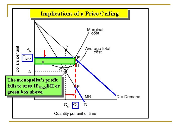
Implications of a Price Ceiling The monopolist’s profit falls to area IPMAXEH or green box above.

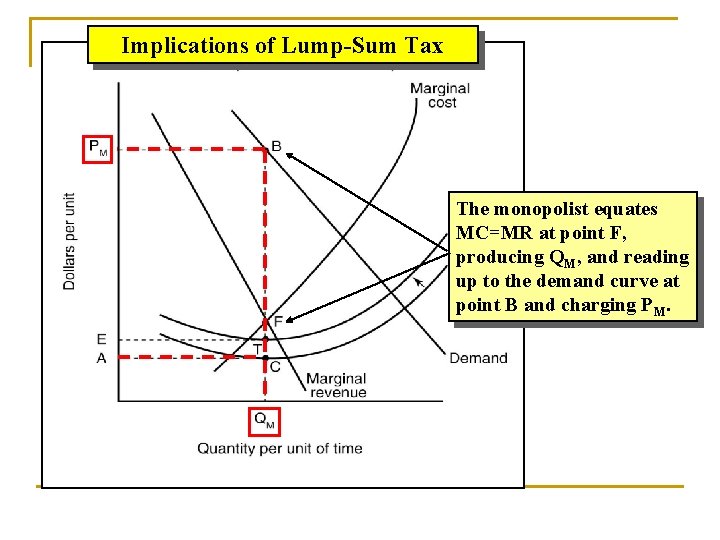
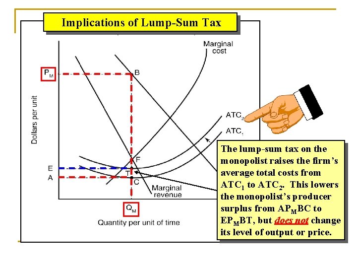
Implications of Lump-Sum Tax The monopolist equates MC=MR at point F, producing QM, and reading up to the demand curve at point B and charging PM.

Implications of Lump-Sum Tax The lump-sum tax on the monopolist raises the firm’s average total costs from ATC 1 to ATC 2. This lowers the monopolist’s producer surplus from APMBC to EPMBT, but does not change its level of output or price.

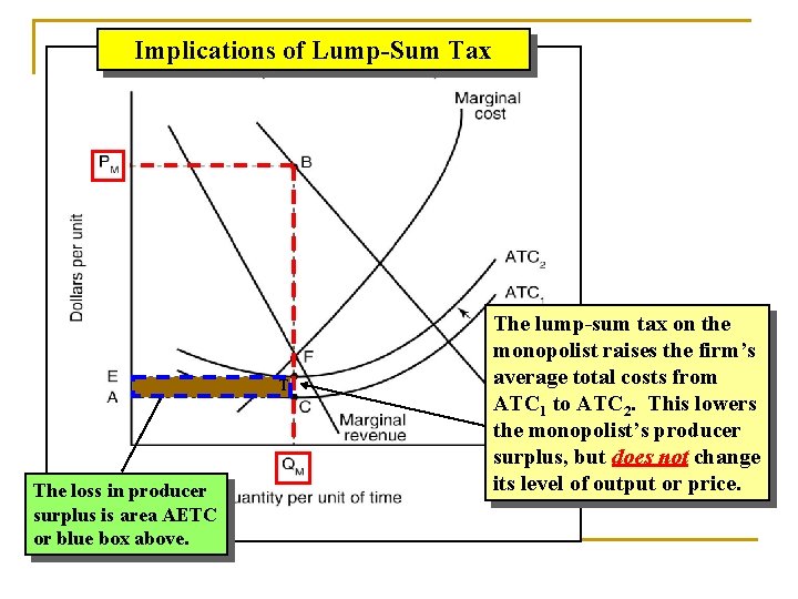
Implications of Lump-Sum Tax T The loss in producer surplus is area AETC or blue box above. The lump-sum tax on the monopolist raises the firm’s average total costs from ATC 1 to ATC 2. This lowers the monopolist’s producer surplus, but does not change its level of output or price.

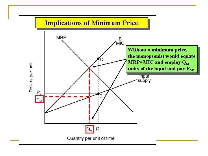
Implications of Minimum Price Without a minimum price, the monopsonist would equate MRP=MIC and employ QM units of the input and pay PM.

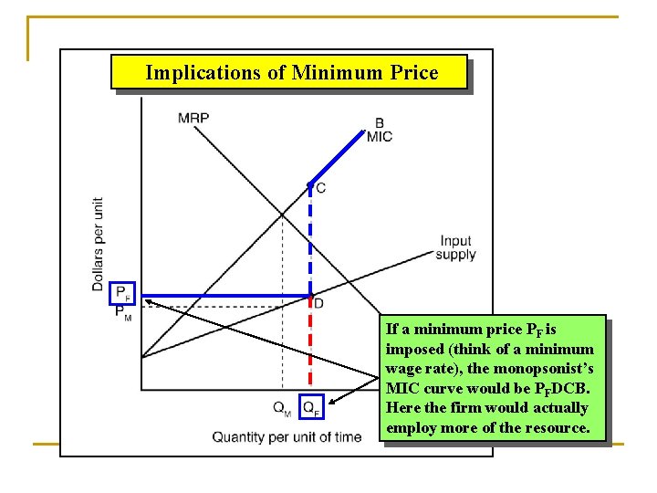
Implications of Minimum Price If a minimum price PF is imposed (think of a minimum wage rate), the monopsonist’s MIC curve would be PFDCB. Here the firm would actually employ more of the resource.

Summary Ø Ø Ø Imperfect competition in the markets which farmers buy production inputs include monopolistic competition, oligopolies and monopolies Imperfect competition in the markets which farmers sell production include monopsonistic competition and oligopsonies Various approaches by the government to modify/control the effects of imperfect competition include regulation and taxation