Aggregation in Dynamic Programming Yu Ashwin Introduction n

Aggregation in Dynamic Programming Yu & Ashwin

Introduction n State aggregation done to reduce computation burdens Since information is lost through state identification, this does not always lead to optimal solution Value = Reduced computation Vs Increased error

Introduction (contd. ) Aggregation Approach n Aggregate the nodes n Solve the aggregated problem n Disaggregate the solution

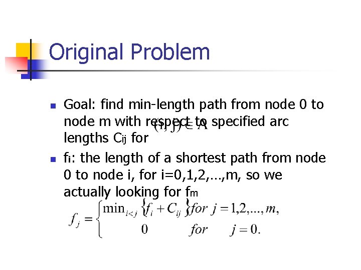
Original Problem n n Goal: find min-length path from node 0 to node m with respect to specified arc lengths Cij for fi: the length of a shortest path from node 0 to node i, for i=0, 1, 2, …, m, so we actually looking for fm

Aggregation n n Notations Entering node Sequential Aggregation Dis-aggregation (SADA) Algorithm Error and bound

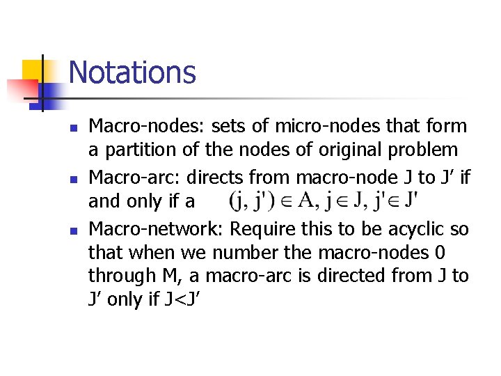
Notations n n n Macro-nodes: sets of micro-nodes that form a partition of the nodes of original problem Macro-arc: directs from macro-node J to J’ if and only if a Macro-network: Require this to be acyclic so that when we number the macro-nodes 0 through M, a macro-arc is directed from J to J’ only if J<J’

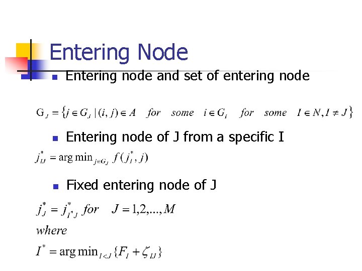
Entering Node n Entering node and set of entering node n Entering node of J from a specific I n Fixed entering node of J

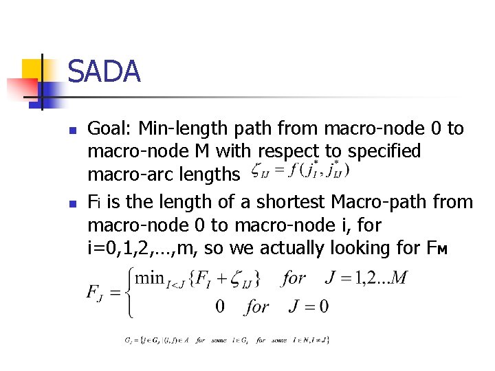
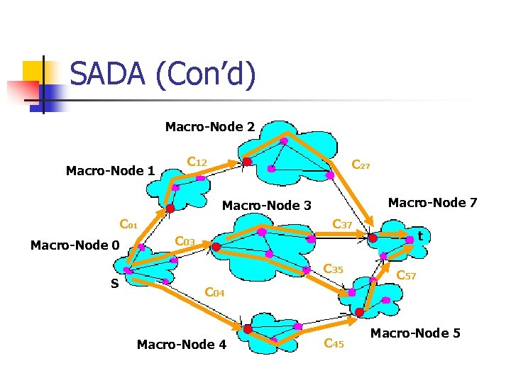
SADA n n Goal: Min-length path from macro-node 0 to macro-node M with respect to specified macro-arc lengths Fi is the length of a shortest Macro-path from macro-node 0 to macro-node i, for i=0, 1, 2, …, m, so we actually looking for FM

SADA (Con’d) Macro-Node 2 Macro-Node 1 C 12 C 27 Macro-Node 3 C 01 Macro-Node 0 S C 37 t C 03 C 35 C 57 C 04 Macro-Node 4 C 45 Macro-Node 5

Concern of Error n n SADA finds the micro-path by construction a shortest path through the micro-network, with the restriction that it must pass through the fixed entering micro-nodes. This may not give the optimal result for the original problem

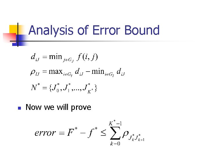
Analysis of Error Bound n Now we will prove

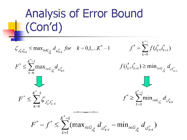
Analysis of Error Bound (Con’d)

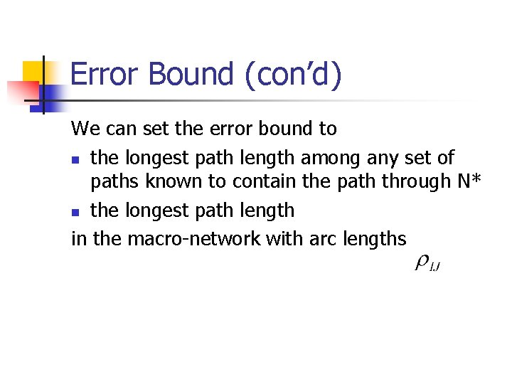
Error Bound (con’d) We can set the error bound to n the longest path length among any set of paths known to contain the path through N* n the longest path length in the macro-network with arc lengths

Benefits of SADA n Computational savings if not all entering micro-nodes of a macro-node are accessible from the fixed entering micro -node of that macro-node

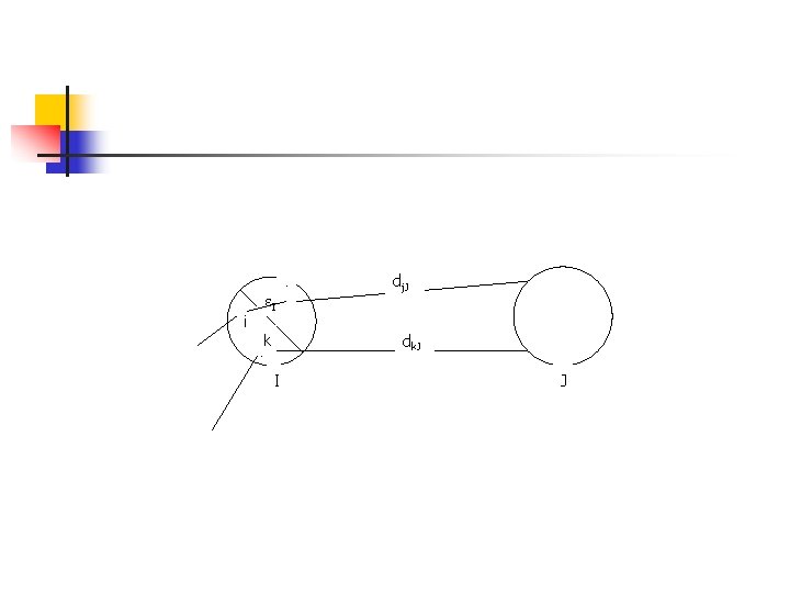
Corollary #3 Let I є N be any macronode and let J є N be any adjacent macronode, so that (I, J) є A. Suppose for any i є GI, there is a j є GI U GJ, with f(i, j) ≤ εI , for some εI ≥ 0 and dk. J ≥ dj. J for all k є GI Then F* – f*≤ ε, where ε is the maximum path length in the macroarc network with zero arc lengths and node penalties εJ for J є N.

i εI j dj. J dk. J k I J

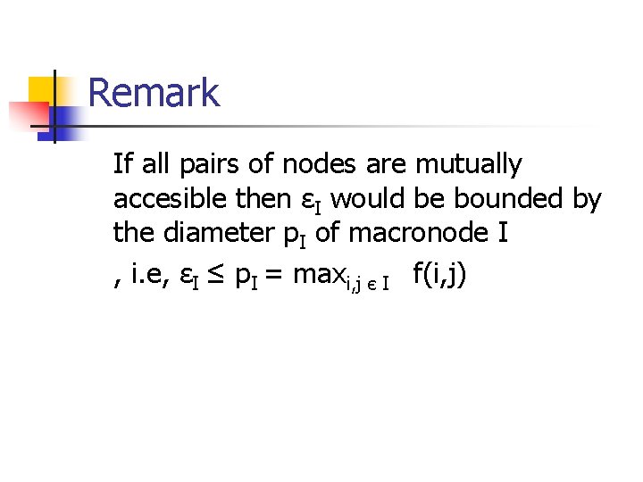
Remark If all pairs of nodes are mutually accesible then εI would be bounded by the diameter p. I of macronode I , i. e, εI ≤ p. I = maxi, j є I f(i, j)

Block staging We can avoid the task solving a longest path problem in finding error bounds in the important special case that the network contains a single macropath from 0 to node M.

Applications to infinite Horizon otpimization We have a acyclic infinite network (N, A) with time ti associated with each node i. The nodes are numbered from 0 to N-1, such that (i, j) є A only if ti<tj, with t 0 = 0. Let C(i, j) arc cost for each arc (i, j).

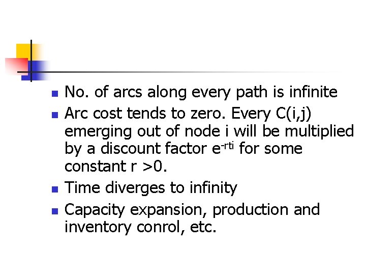
n n No. of arcs along every path is infinite Arc cost tends to zero. Every C(i, j) emerging out of node i will be multiplied by a discount factor e-rti for some constant r >0. Time diverges to infinity Capacity expansion, production and inventory conrol, etc.

n n n Such problems are solved by truncating them to a finite length problem of T periods. The resulting problem is solved by standard dynamic programming Under mild regulations, this procedure for large enough T will result in optimal initial arc decision that is optimal for infinite horizon problem

n n A sufficiently large T is difficult to identify. All data must be first forecasted over infinite horizon For an ε error the planner willing to accept, then an approximate horizon length Tε* can be determined

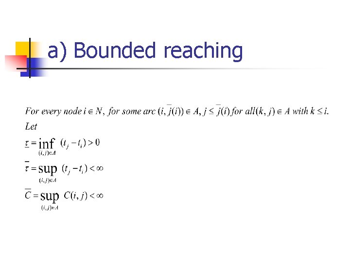
a) Bounded reaching

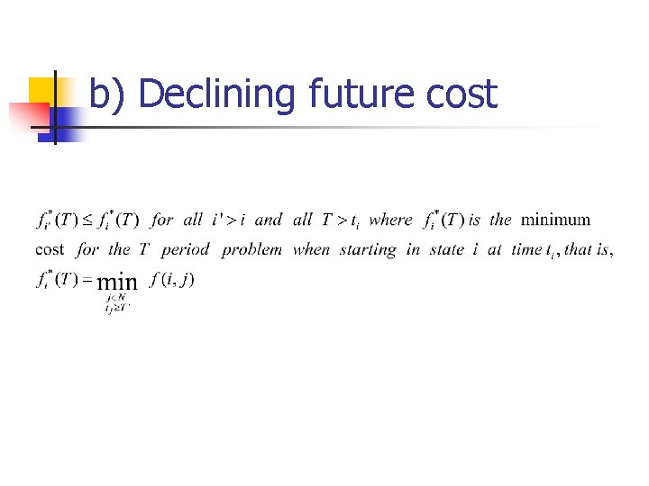
b) Declining future cost

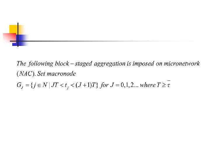
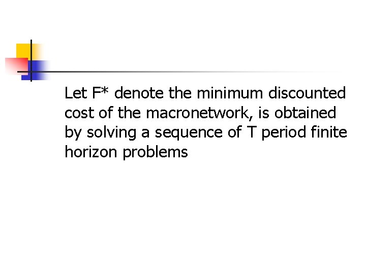
Let F* denote the minimum discounted cost of the macronetwork, is obtained by solving a sequence of T period finite horizon problems

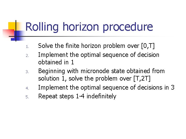
Rolling horizon procedure 1. 2. 3. 4. 5. Solve the finite horizon problem over [0, T] Implement the optimal sequence of decision obtained in 1 Beginning with micronode state obtained from solution 1, solve the problem over [T, 2 T] Implement the optimal sequence of decisions in 3 Repeat steps 1 -4 indefinitely

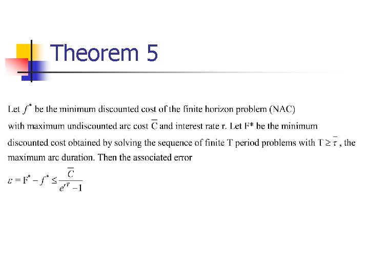
Theorem 5

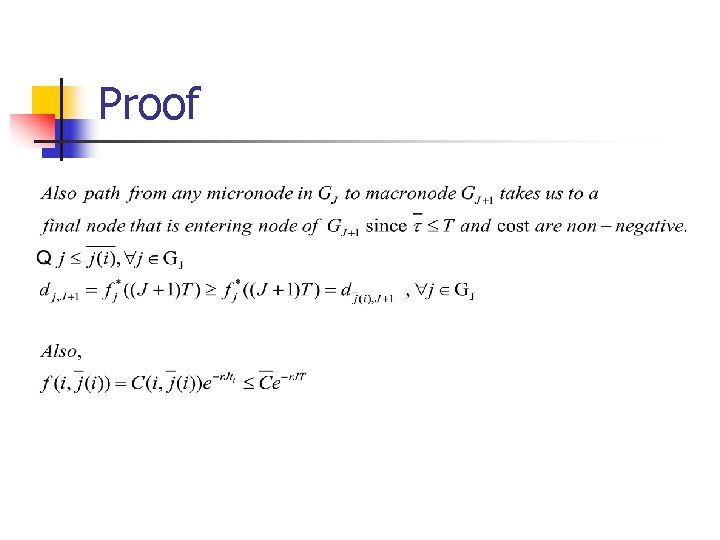
Proof

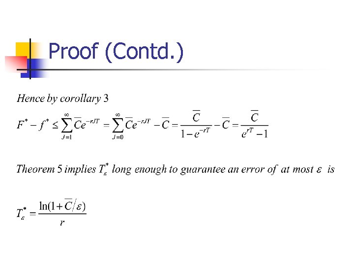
Proof (Contd. )