Aggregate Planning 1 The Role of the Aggregate

Aggregate Planning 1

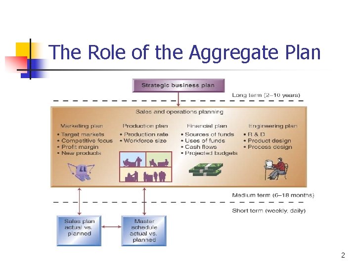
The Role of the Aggregate Plan 2

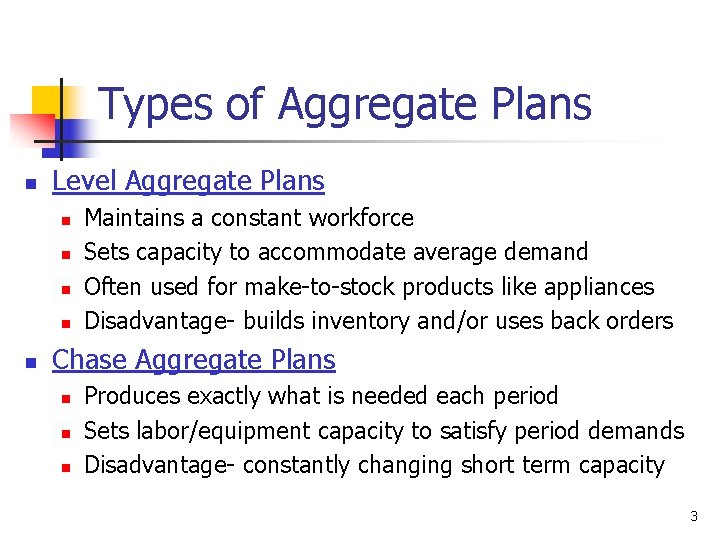
Types of Aggregate Plans n Level Aggregate Plans n n n Maintains a constant workforce Sets capacity to accommodate average demand Often used for make-to-stock products like appliances Disadvantage- builds inventory and/or uses back orders Chase Aggregate Plans n n n Produces exactly what is needed each period Sets labor/equipment capacity to satisfy period demands Disadvantage- constantly changing short term capacity 3

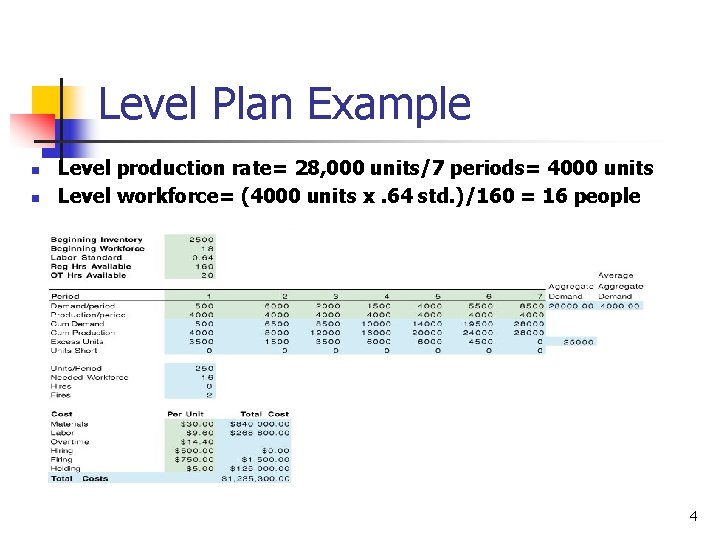
Level Plan Example n n Level production rate= 28, 000 units/7 periods= 4000 units Level workforce= (4000 units x. 64 std. )/160 = 16 people 4

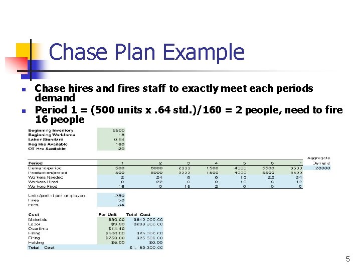
Chase Plan Example n n Chase hires and fires staff to exactly meet each periods demand Period 1 = (500 units x. 64 std. )/160 = 2 people, need to fire 16 people 5

Types of Aggregate Plans n (Cont. ) Hybrid Aggregate Plans n Uses a combination of options n Options should be limited to facilitate execution n May use a level workforce with overtime & temps n May allow inventory buildup and some backordering n May use short term sourcing 6

Aggregate Planning Options n Demand based options n n n Reactive: uses finished goods inventories and backorders for fluctuations Proactive: shifting the demand patterns to minimize fluctuations e. g. early bird dinner prices at a restaurant Capacity based options n n Changes output capacity to meet demand Uses overtime, undertime, subcontracting, hiring, firing, and part-timers – cost and operational implications 7

Starting with the Current Situation n Point of Departure n n n Magnitude of change n n Current % of normal capacity Options are different depending on present situation Larger changes need more dramatic measures Duration of change n n Is the length of time a brief seasonal change? Is a permanent change in capacity needed? 8

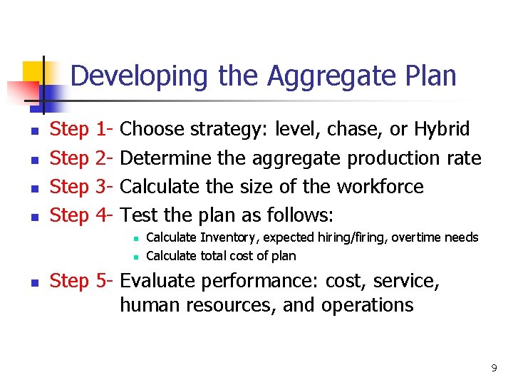
Developing the Aggregate Plan n n Step 1234 - Choose strategy: level, chase, or Hybrid Determine the aggregate production rate Calculate the size of the workforce Test the plan as follows: n n n Calculate Inventory, expected hiring/firing, overtime needs Calculate total cost of plan Step 5 - Evaluate performance: cost, service, human resources, and operations 9

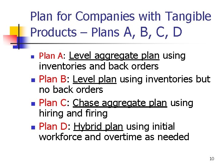
Plan for Companies with Tangible Products – Plans A, B, C, D n n Plan A: Level aggregate plan using inventories and back orders Plan B: Level plan using inventories but no back orders Plan C: Chase aggregate plan using hiring and firing Plan D: Hybrid plan using initial workforce and overtime as needed 10

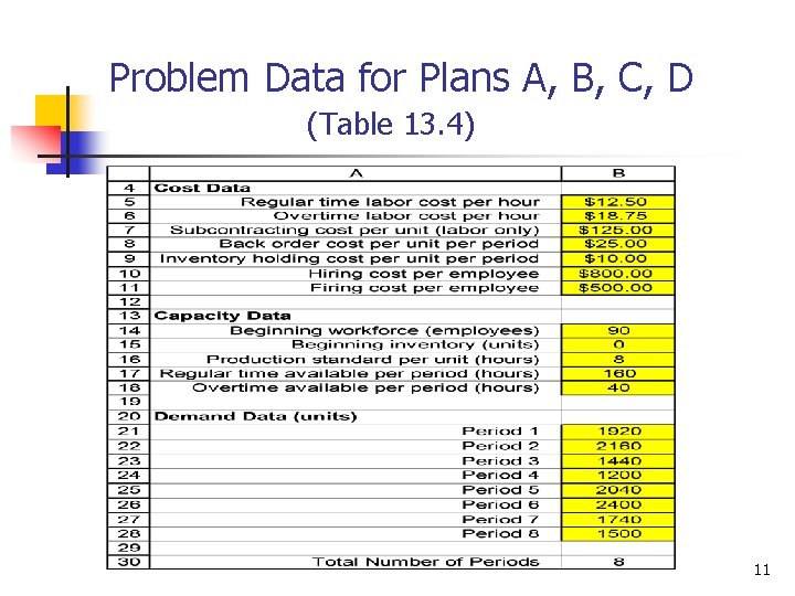
Problem Data for Plans A, B, C, D (Table 13. 4) 11

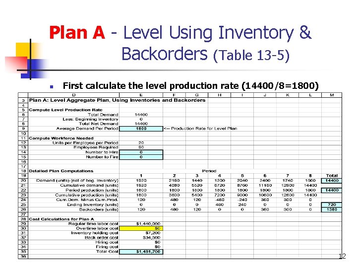
Plan A - Level Using Inventory & Backorders (Table 13 -5) n First calculate the level production rate (14400/8=1800) 12

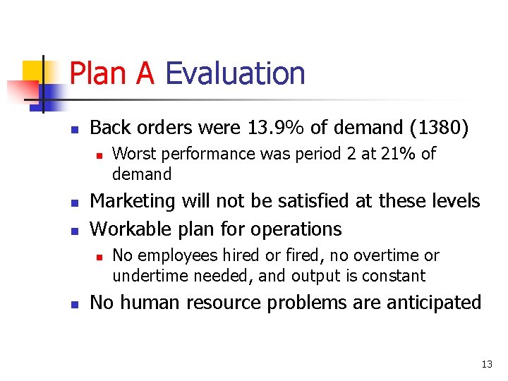
Plan A Evaluation n Back orders were 13. 9% of demand (1380) n n n Marketing will not be satisfied at these levels Workable plan for operations n n Worst performance was period 2 at 21% of demand No employees hired or fired, no overtime or undertime needed, and output is constant No human resource problems are anticipated 13

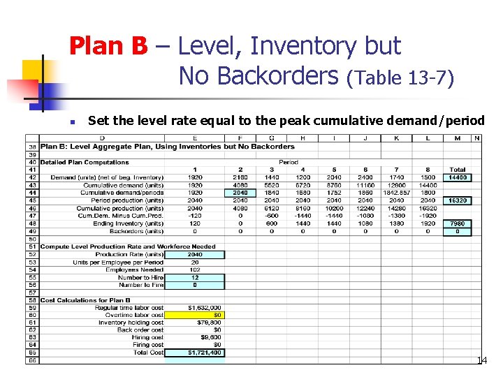
Plan B – Level, Inventory but No Backorders (Table 13 -7) n Set the level rate equal to the peak cumulative demand/period 14

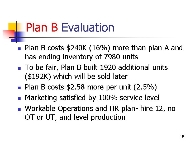
Plan B Evaluation n n Plan B costs $240 K (16%) more than plan A and has ending inventory of 7980 units To be fair, Plan B built 1920 additional units ($192 K) which will be sold later Plan B costs $2. 58 more per unit (2. 5%) Marketing satisfied by 100% service level Workable Operations and HR plan- hire 12, no OT or UT, and level production 15

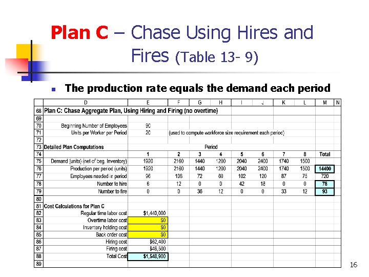
Plan C – Chase Using Hires and Fires (Table 13 - 9) n The production rate equals the demand each period 16

Plan C Evaluation n Costs an additional $2 per unit more than Plan B Marketing is satisfied again by 100% service level From Operations and HR standpoint, not easy to implement: n n n Need space, tools, equipment for up to 120 people in period 6 and only have 60 people in period 4 High training costs and potential quality problems Low morale likely due to poor job security 17

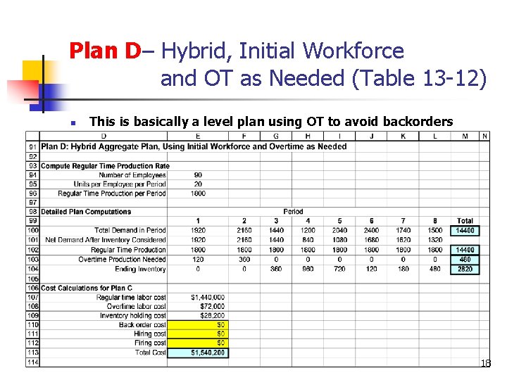
Plan D– Hybrid, Initial Workforce and OT as Needed (Table 13 -12) n This is basically a level plan using OT to avoid backorders 18

Plan D Evaluation n n Cost is only $. 61 (. 6%) more than Plan A with a reasonable increase in ending inventory (+1440) Marketing is satisfied as well with 100% service level n Not difficult for Operations to implement n Does not need excessive overtime n n Uses overtime in just periods 1 and 2 (7%, 20%) Aggregate Plan Objective: Keep customer service high and costs low 19

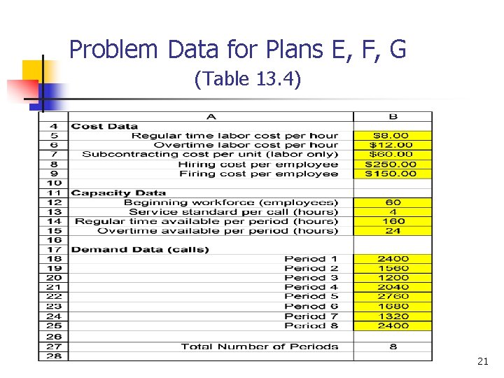
Aggregate Plans for Service Companies with Non-Tangible Products- Plans E, F, G n Options remain the same – level, chase, and hybrid plans n n Overtime and undertime can be used Staff can be hired and fired Inventory cannot be used to level the service plan All demand must be satisfied or lose business to a competing service provider 20

Problem Data for Plans E, F, G (Table 13. 4) 21

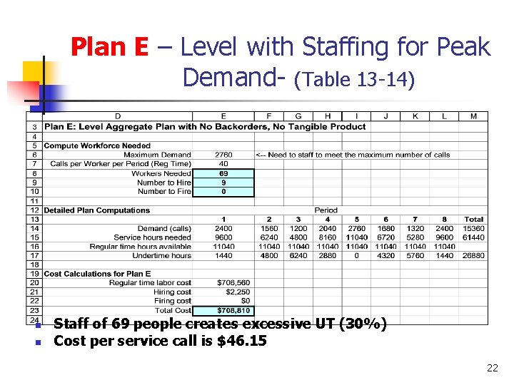
Plan E – Level with Staffing for Peak Demand- (Table 13 -14) n n Staff of 69 people creates excessive UT (30%) Cost per service call is $46. 15 22

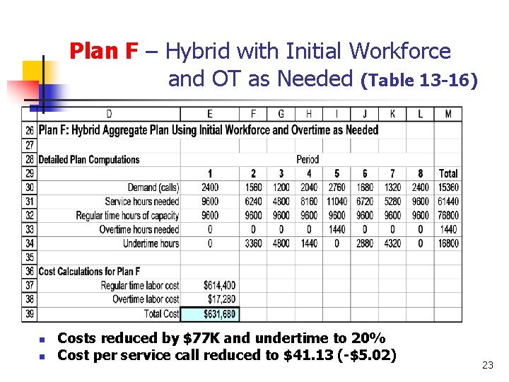
Plan F – Hybrid with Initial Workforce and OT as Needed (Table 13 -16) n n Costs reduced by $77 K and undertime to 20% Cost per service call reduced to $41. 13 (-$5. 02) 23

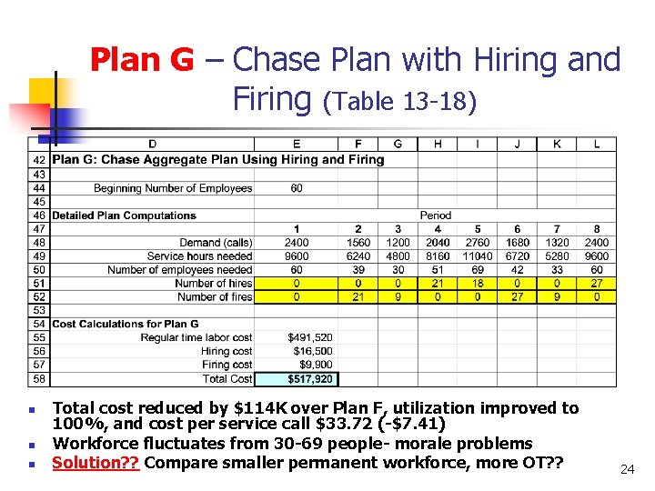
Plan G – Chase Plan with Hiring and Firing (Table 13 -18) n n n Total cost reduced by $114 K over Plan F, utilization improved to 100%, and cost per service call $33. 72 (-$7. 41) Workforce fluctuates from 30 -69 people- morale problems Solution? ? Compare smaller permanent workforce, more OT? ? 24

Aggregate Planning Bottom Line n n n The Aggregate plan must balance several perspectives Costs are important but so are: n Customer service n Operational effectiveness n Workforce morale A successful AP considers each of these factors 25

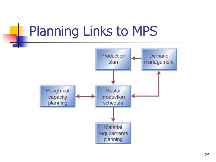
Planning Links to MPS 26

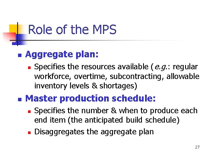
Role of the MPS n Aggregate plan: n n Specifies the resources available (e. g. : regular workforce, overtime, subcontracting, allowable inventory levels & shortages) Master production schedule: n n Specifies the number & when to produce each end item (the anticipated build schedule) Disaggregates the aggregate plan 27

Objectives of Master Schedule n The Master Scheduler must: n n Maintain the desired customer service level Utilize resources efficiently Maintain desired inventory levels The Master Schedule must: n n n Satisfy customer demand Not exceed Operation’s capacity Work within the constraints of the Aggregate Plan 28

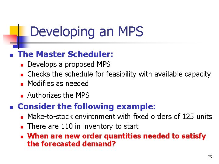
Developing an MPS n The Master Scheduler: n Develops a proposed MPS Checks the schedule for feasibility with available capacity Modifies as needed n Authorizes the MPS n n n Consider the following example: n n n Make-to-stock environment with fixed orders of 125 units There are 110 in inventory to start When are new order quantities needed to satisfy the forecasted demand? 29

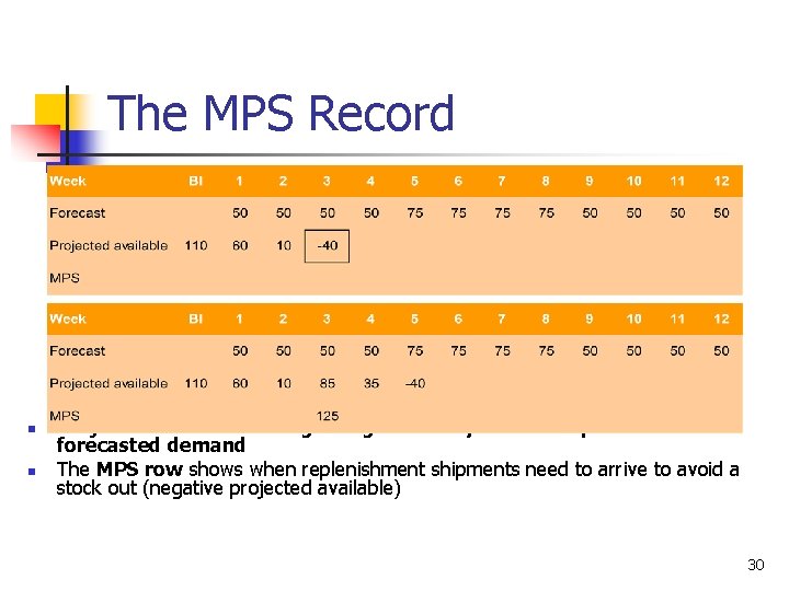
The MPS Record n n Projected Available = beginning inventory + MPS shipments forecasted demand The MPS row shows when replenishment shipments need to arrive to avoid a stock out (negative projected available) 30

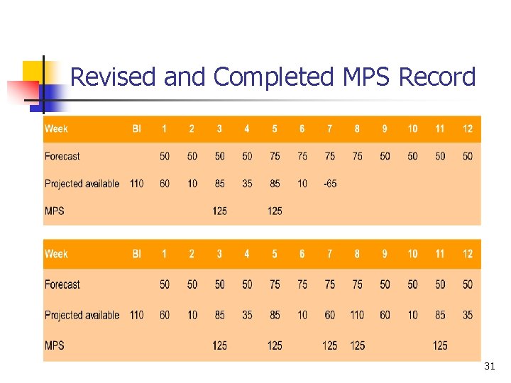
Revised and Completed MPS Record 31

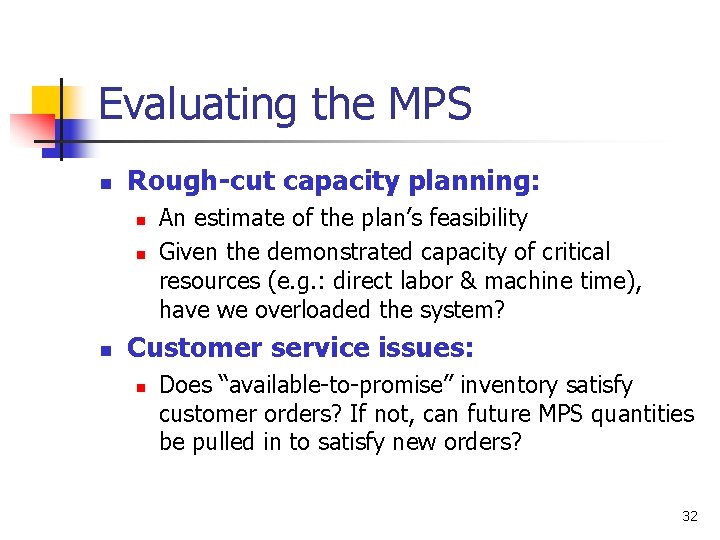
Evaluating the MPS n Rough-cut capacity planning: n n n An estimate of the plan’s feasibility Given the demonstrated capacity of critical resources (e. g. : direct labor & machine time), have we overloaded the system? Customer service issues: n Does “available-to-promise” inventory satisfy customer orders? If not, can future MPS quantities be pulled in to satisfy new orders? 32

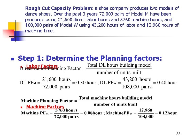
Rough Cut Capacity Problem: a shoe company produces two models of dance shoes. Over the past 3 years 72, 000 pairs of Model M have been produced using 21, 600 direct labor hours and 5760 machine hours, and 108, 000 pairs of Model W using 43, 200 hours of labor and 12, 960 hours of machine time. n Step 1: Determine the Planning factors: n Labor Factors n Machine Factors 33

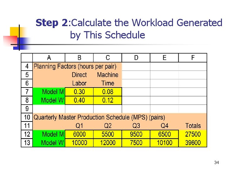
Step 2: Calculate the Workload Generated by This Schedule 34

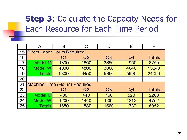
Step 3: Calculate the Capacity Needs for Each Resource for Each Time Period 35

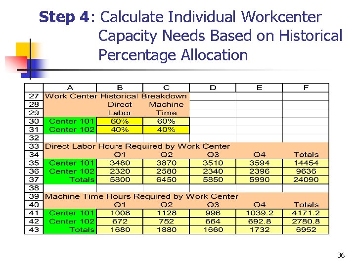
Step 4: Calculate Individual Workcenter Capacity Needs Based on Historical Percentage Allocation 36

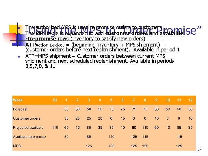
n n Using the MPS to “Order Promise” The authorized MPS is used to promise orders to customers The MPS table is expanded to add customer orders and available -to-promise rows (inventory to satisfy new orders) ATPAction Bucket = (beginning inventory + MPS shipment) – (customer orders before next replenishment). Available in period 1 ATP=MPS shipment – Customer orders between current MPS shipment and next scheduled replenishment. Available in periods 3, 5, 7, 8, & 11 37

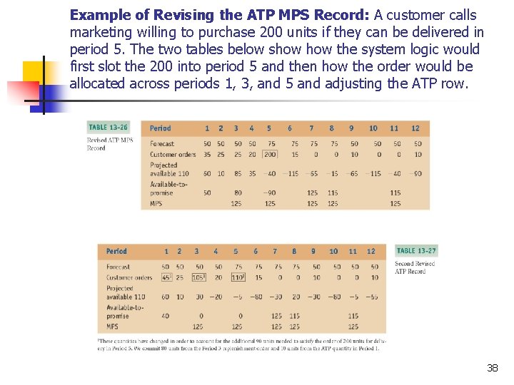
Example of Revising the ATP MPS Record: A customer calls marketing willing to purchase 200 units if they can be delivered in period 5. The two tables below show the system logic would first slot the 200 into period 5 and then how the order would be allocated across periods 1, 3, and 5 and adjusting the ATP row. 38

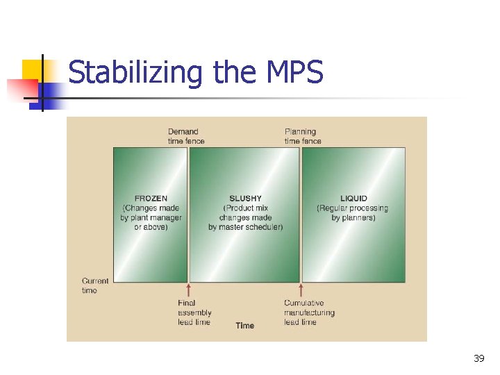
Stabilizing the MPS 39