Aggregate Function Computation and Iceberg Querying in Vertical

Aggregate Function Computation and Iceberg Querying in Vertical Databases Yue (Jenny) Cui Advisor: Dr. William Perrizo Master Thesis Oral Defense Department of Computer Science North Dakota State University

Outline o Introduction n Review of Aggregate Functions n Review of Iceberg Queries o Algorithms of Aggregate Function Computation Using P-trees n SUM, COUNT, and AVERAGE. n MAX, MIN, MEDIAN, RANK, and TOP-K. o Iceberg Query Operation Using P-trees n An Iceberg Query Example o Performance Analysis o Conclusion

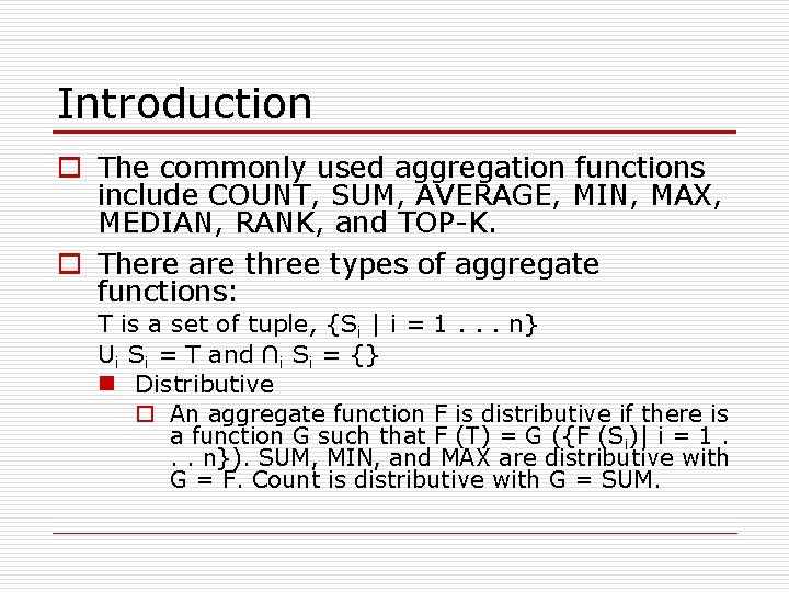
Introduction o The commonly used aggregation functions include COUNT, SUM, AVERAGE, MIN, MAX, MEDIAN, RANK, and TOP-K. o There are three types of aggregate functions: T is a set of tuple, {Si | i = 1. . . n} Ui Si = T and ∩i Si = {} n Distributive o An aggregate function F is distributive if there is a function G such that F (T) = G ({F (Si)| i = 1. . . n}). SUM, MIN, and MAX are distributive with G = F. Count is distributive with G = SUM.

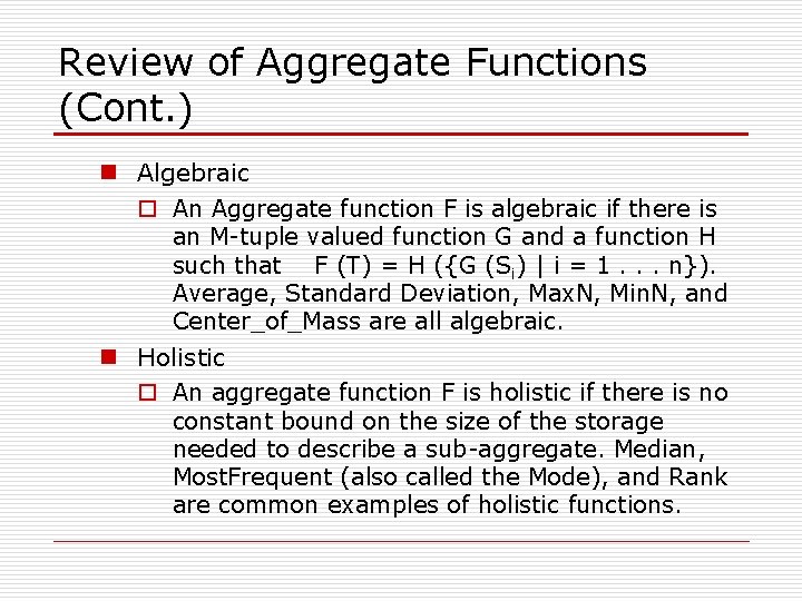
Review of Aggregate Functions (Cont. ) n Algebraic o An Aggregate function F is algebraic if there is an M-tuple valued function G and a function H such that F (T) = H ({G (Si) | i = 1. . . n}). Average, Standard Deviation, Max. N, Min. N, and Center_of_Mass are all algebraic. n Holistic o An aggregate function F is holistic if there is no constant bound on the size of the storage needed to describe a sub-aggregate. Median, Most. Frequent (also called the Mode), and Rank are common examples of holistic functions.

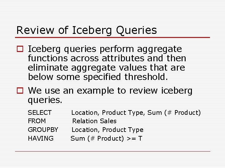
Review of Iceberg Queries o Iceberg queries perform aggregate functions across attributes and then eliminate aggregate values that are below some specified threshold. o We use an example to review iceberg queries. SELECT FROM GROUPBY HAVING Location, Product Type, Sum (# Product) Relation Sales Location, Product Type Sum (# Product) >= T

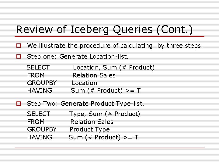
Review of Iceberg Queries (Cont. ) o We illustrate the procedure of calculating by three steps. o Step one: Generate Location-list. SELECT FROM GROUPBY HAVING Location, Sum (# Product) Relation Sales Location Sum (# Product) >= T o Step Two: Generate Product Type-list. SELECT FROM GROUPBY HAVING Type, Sum (# Product) Relation Sales Product Type Sum (# Product) >= T

Review of Iceberg Queries (Cont. ) o Step Three: Generate location & Product Type pair groups. o From the Location-list and the Type-list we generated in first two steps, we can eliminate many of the location & Product Type pair groups according to the threshold T.

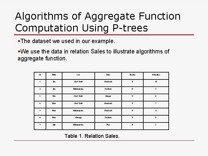
Algorithms of Aggregate Function Computation Using P-trees §The dataset we used in our example. §We use the data in relation Sales to illustrate algorithms of aggregate function. Id Mon Loc Type On line # Product 1 Jan New York Notebook Y 10 2 Jan Minneapolis Desktop N 5 3 Feb New York Printer Y 6 4 Mar New York Notebook Y 7 5 Mar Minneapolis Notebook Y 11 6 Mar Chicago Desktop Y 9 7 Apr Minneapolis Fax N 3 Table 1. Relation Sales.

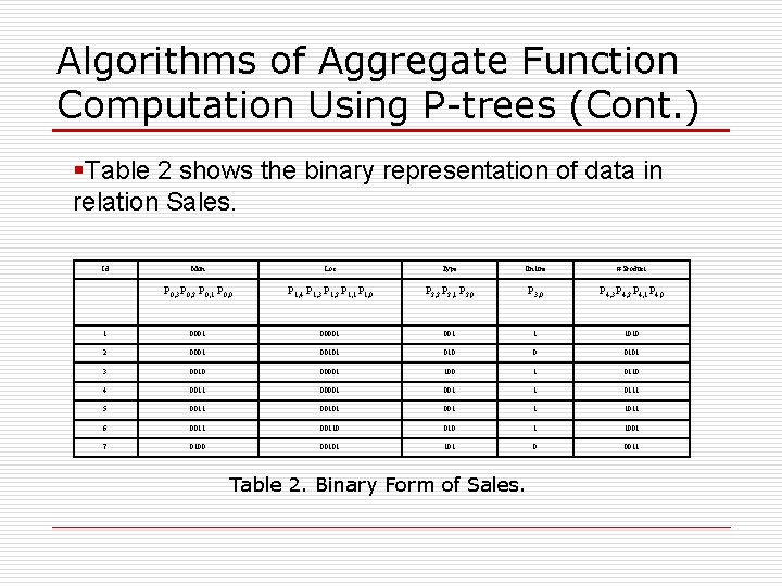
Algorithms of Aggregate Function Computation Using P-trees (Cont. ) §Table 2 shows the binary representation of data in relation Sales. Id Mon Loc Type On line # Product P 0, 3 P 0, 2 P 0, 1 P 0, 0 P 1, 4 P 1, 3 P 1, 2 P 1, 1 P 1, 0 P 2, 2 P 2, 1 P 2, 0 P 3, 0 P 4, 3 P 4, 2 P 4, 1 P 4, 0 1 00001 001 1 1010 2 0001 00101 010 0 0101 3 0010 00001 100 1 0110 4 0011 00001 1 0111 5 0011 00101 001 1 1011 6 00110 010 1 1001 7 0100 00101 0 0011 Table 2. Binary Form of Sales.

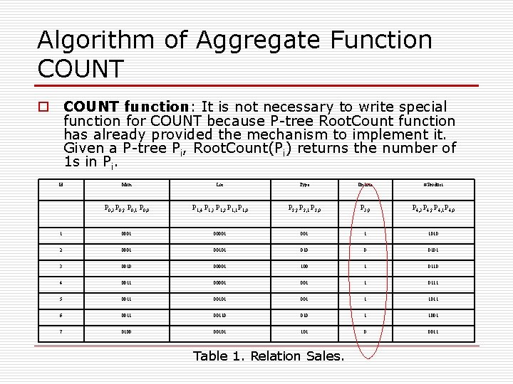
Algorithm of Aggregate Function COUNT o COUNT function: It is not necessary to write special function for COUNT because P-tree Root. Count function has already provided the mechanism to implement it. Given a P-tree Pi, Root. Count(Pi) returns the number of 1 s in Pi. Id Mon Loc Type On line # Product P 0, 3 P 0, 2 P 0, 1 P 0, 0 P 1, 4 P 1, 3 P 1, 2 P 1, 1 P 1, 0 P 2, 2 P 2, 1 P 2, 0 P 3, 0 P 4, 3 P 4, 2 P 4, 1 P 4, 0 1 00001 001 1 1010 2 0001 00101 010 0 0101 3 0010 00001 100 1 0110 4 0011 00001 1 0111 5 0011 00101 001 1 1011 6 00110 010 1 1001 7 0100 00101 0 0011 Table 1. Relation Sales.

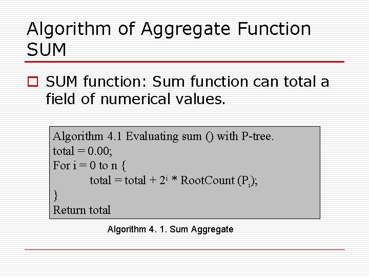
Algorithm of Aggregate Function SUM o SUM function: Sum function can total a field of numerical values. Algorithm 4. 1 Evaluating sum () with P-tree. total = 0. 00; For i = 0 to n { total = total + 2 i * Root. Count (Pi); } Return total Algorithm 4. 1. Sum Aggregate

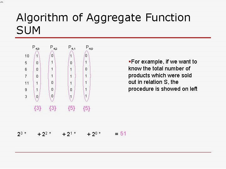
Algorithm of Aggregate Function SUM P 4, 3 P 4, 2 P 4, 1 P 4, 0 10 1 0 5 0 1 6 0 1 1 0 7 0 1 11 1 0 1 1 9 1 0 0 1 3 0 0 1 1 {3} {5} 23 * + 22 * + 21 * + 20 * §For example, if we want to know the total number of products which were sold out in relation S, the procedure is showed on left = 51

Algorithm of Aggregate Function AVERAGE o Average function: Average function will show the average value in a field. It can be calculated from function COUNT and SUM. Average () = Sum ()/Count ().

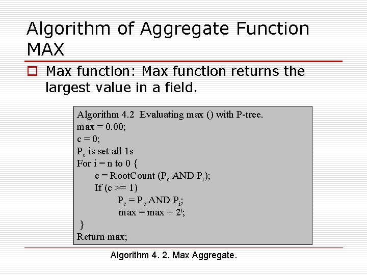
Algorithm of Aggregate Function MAX o Max function: Max function returns the largest value in a field. Algorithm 4. 2 Evaluating max () with P-tree. max = 0. 00; c = 0; Pc is set all 1 s For i = n to 0 { c = Root. Count (Pc AND Pi); If (c >= 1) Pc = Pc AND Pi; max = max + 2 i; } Return max; Algorithm 4. 2. Max Aggregate.

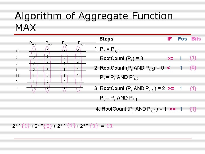
Algorithm of Aggregate Function MAX P 4, 3 P 4, 2 P 4, 1 P 4, 0 10 1 0 5 0 1 6 0 1 1 0 7 0 1 11 1 0 1 1 9 1 0 0 1 3 0 0 1 1 Steps IF Pos Bits >= 1 {1} 1 {0} 1 {1} 4. Root. Count (Pc AND P 4, 0 ) = 1 >= 1 {1} 1. Pc = P 4, 3 Root. Count (Pc) = 3 2. Root. Count (Pc AND P 4, 2) = 0 < Pc = Pc AND P’ 4, 2 3. Root. Count (Pc AND P 4, 1 ) = 2 >= Pc AND P 4, 1 23 * {1}+ 22 *{0}+ 21 * {1}+ 20 * {1} = 11

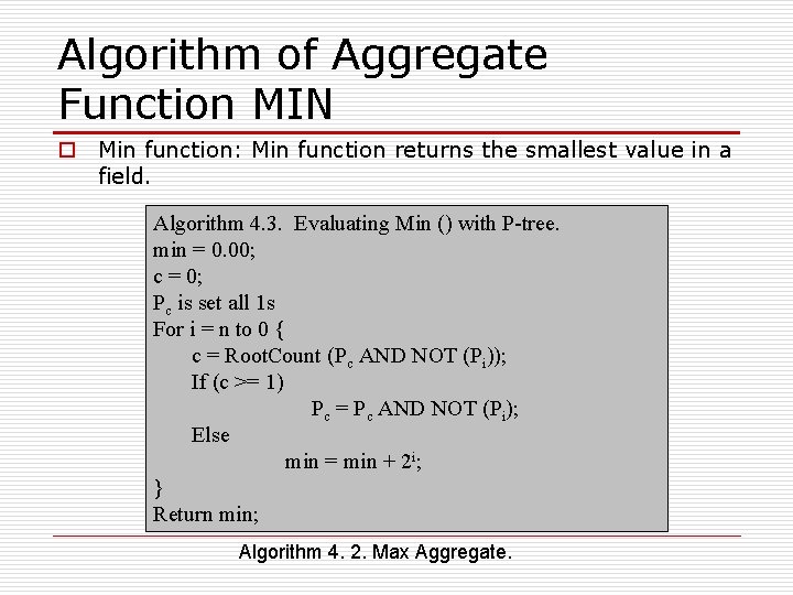
Algorithm of Aggregate Function MIN o Min function: Min function returns the smallest value in a field. Algorithm 4. 3. Evaluating Min () with P-tree. min = 0. 00; c = 0; Pc is set all 1 s For i = n to 0 { c = Root. Count (Pc AND NOT (Pi)); If (c >= 1) Pc = Pc AND NOT (Pi); Else min = min + 2 i; } Return min; Algorithm 4. 2. Max Aggregate.

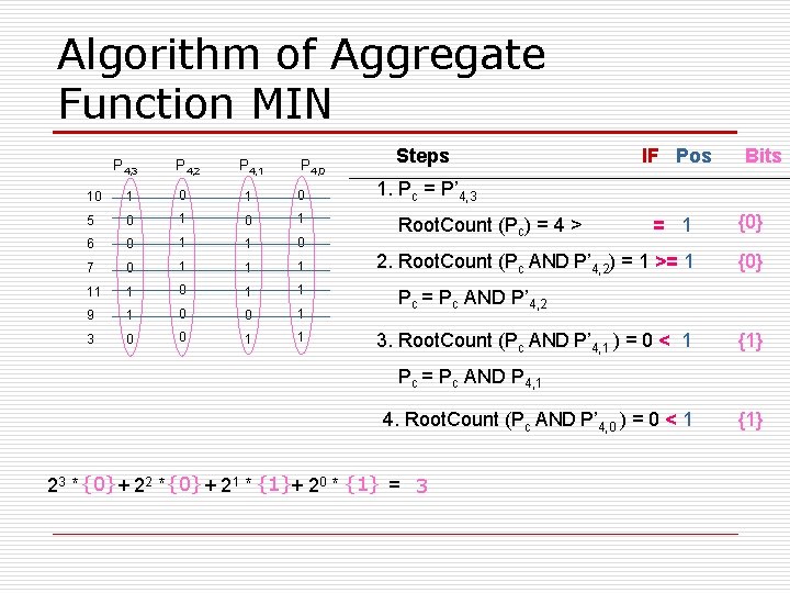
Algorithm of Aggregate Function MIN P 4, 3 P 4, 2 P 4, 1 P 4, 0 10 1 0 5 0 1 6 0 1 1 0 7 0 1 11 1 0 1 1 9 1 0 0 1 3 0 0 1 1 Steps IF Pos Bits 1. Pc = P’ 4, 3 = 1 {0} 2. Root. Count (Pc AND P’ 4, 2) = 1 >= 1 {0} Root. Count (Pc) = 4 > Pc = Pc AND P’ 4, 2 3. Root. Count (Pc AND P’ 4, 1 ) = 0 < 1 {1} Pc = Pc AND P 4, 1 4. Root. Count (Pc AND P’ 4, 0 ) = 0 < 1 23 * {0}+ 22 *{0}+ 21 * {1}+ 20 * {1} = 3 {1}

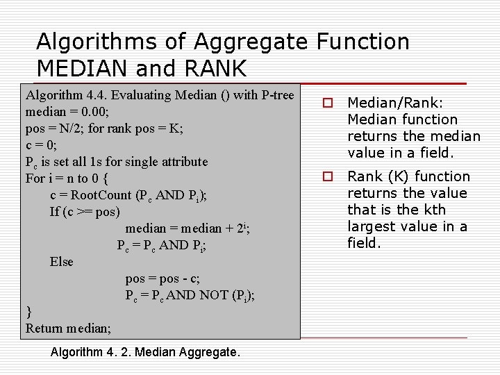
Algorithms of Aggregate Function MEDIAN and RANK Algorithm 4. 4. Evaluating Median () with P-tree median = 0. 00; pos = N/2; for rank pos = K; c = 0; Pc is set all 1 s for single attribute For i = n to 0 { c = Root. Count (Pc AND Pi); If (c >= pos) median = median + 2 i; Pc = Pc AND Pi; Else pos = pos - c; Pc = Pc AND NOT (Pi); } Return median; Algorithm 4. 2. Median Aggregate. o Median/Rank: Median function returns the median value in a field. o Rank (K) function returns the value that is the kth largest value in a field.

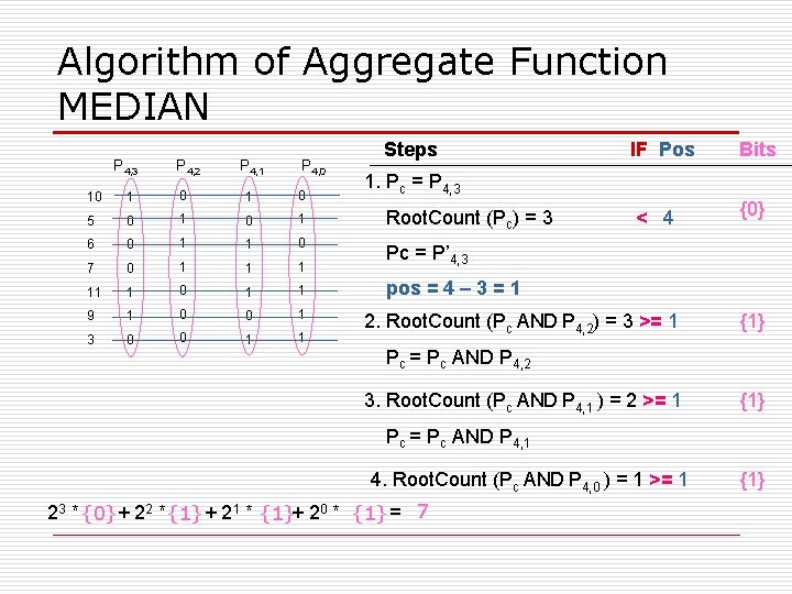
Algorithm of Aggregate Function MEDIAN P 4, 3 P 4, 2 P 4, 1 P 4, 0 Steps IF Pos Bits < 4 {0} 2. Root. Count (Pc AND P 4, 2) = 3 >= 1 {1} 1. Pc = P 4, 3 10 1 0 5 0 1 Root. Count (Pc) = 3 6 0 1 1 0 7 0 1 1 1 Pc = P’ 4, 3 11 1 0 1 1 9 1 0 0 1 1 3 pos = 4 – 3 = 1 Pc = Pc AND P 4, 2 3. Root. Count (Pc AND P 4, 1 ) = 2 >= 1 {1} Pc = Pc AND P 4, 1 4. Root. Count (Pc AND P 4, 0 ) = 1 >= 1 23 * {0}+ 22 *{1}+ 21 * {1}+ 20 * {1} = 7 {1}

Algorithm of Aggregate Function TOP-K o Top-k function: In order to get the largest k values in a field, first, we will find rank k value Vk using function Rank (K). o Second, we will find all the tuples whose values are greater than or equal to Vk. Using ENRING technology of P-tree

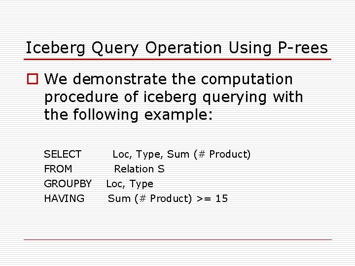
Iceberg Query Operation Using P-rees o We demonstrate the computation procedure of iceberg querying with the following example: SELECT FROM GROUPBY HAVING Loc, Type, Sum (# Product) Relation S Loc, Type Sum (# Product) >= 15

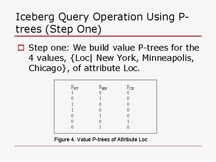
Iceberg Query Operation Using Ptrees (Step One) o Step one: We build value P-trees for the 4 values, {Loc| New York, Minneapolis, Chicago}, of attribute Loc. PNY 1 0 1 1 0 0 0 PMN 0 1 0 1 PCH 0 0 0 1 0 Figure 4. Value P-trees of Attribute Loc

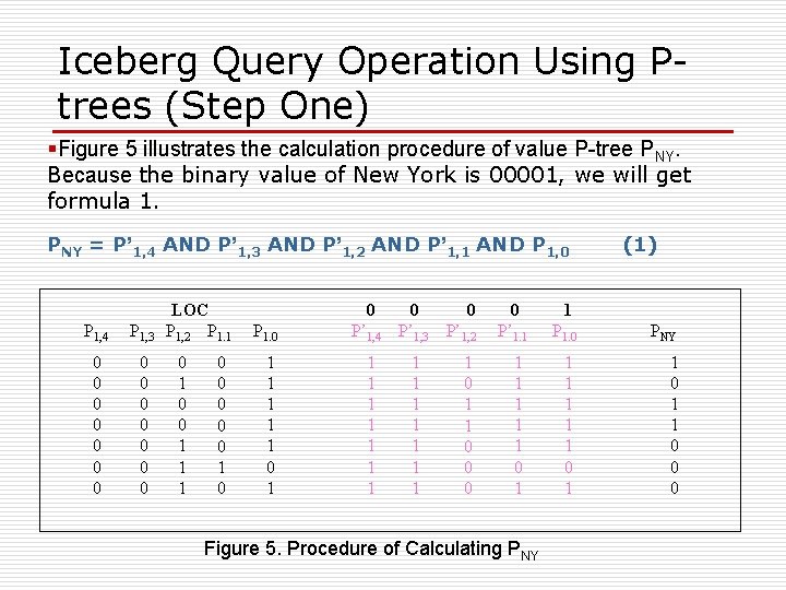
Iceberg Query Operation Using Ptrees (Step One) §Figure 5 illustrates the calculation procedure of value P-tree PNY. Because the binary value of New York is 00001, we will get formula 1. PNY = P’ 1, 4 AND P’ 1, 3 AND P’ 1, 2 AND P’ 1, 1 AND P 1, 0 P 1, 4 P 1, 3 0 0 0 0 LOC P 1, 2 P 1. 1 0 0 1 1 1 0 0 0 1 0 P 1. 0 1 1 1 0 0 0 P’ 1, 4 P’ 1, 3 P’ 1, 2 1 1 1 1 0 1 1 0 0 0 (1) 0 P’ 1. 1 P 1. 0 PNY 1 1 1 1 1 0 1 1 0 0 0 Figure 5. Procedure of Calculating PNY 1

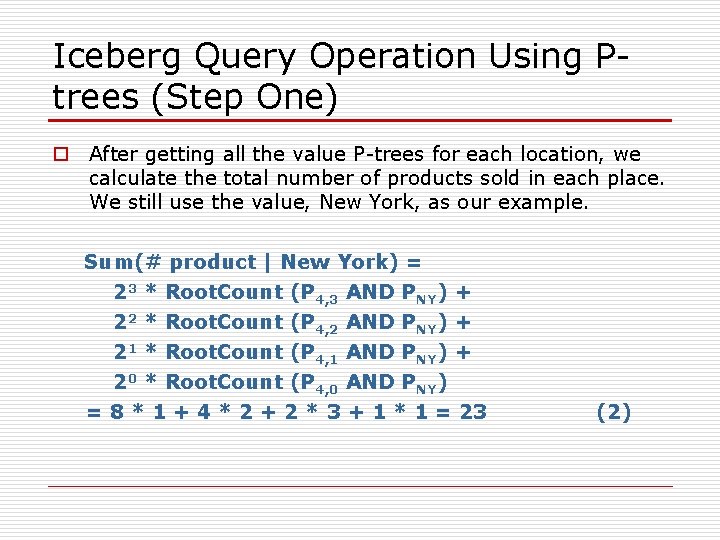
Iceberg Query Operation Using Ptrees (Step One) o After getting all the value P-trees for each location, we calculate the total number of products sold in each place. We still use the value, New York, as our example. Sum(# product | New York) = 23 * Root. Count (P 4, 3 AND PNY) + 22 * Root. Count (P 4, 2 AND PNY) + 21 * Root. Count (P 4, 1 AND PNY) + 20 * Root. Count (P 4, 0 AND PNY) = 8 * 1 + 4 * 2 + 2 * 3 + 1 * 1 = 23 (2)

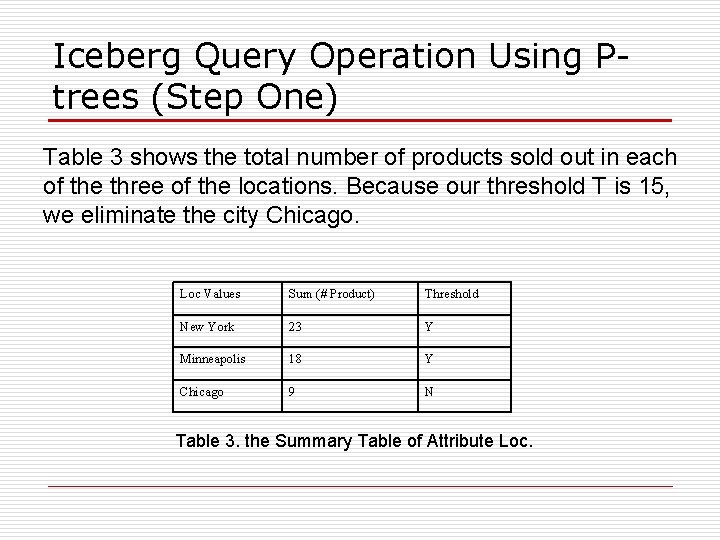
Iceberg Query Operation Using Ptrees (Step One) Table 3 shows the total number of products sold out in each of the three of the locations. Because our threshold T is 15, we eliminate the city Chicago. Loc Values Sum (# Product) Threshold New York 23 Y Minneapolis 18 Y Chicago 9 N Table 3. the Summary Table of Attribute Loc.

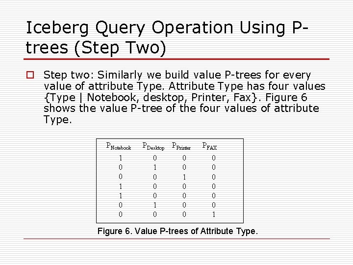
Iceberg Query Operation Using Ptrees (Step Two) o Step two: Similarly we build value P-trees for every value of attribute Type. Attribute Type has four values {Type | Notebook, desktop, Printer, Fax}. Figure 6 shows the value P-tree of the four values of attribute Type. PNotebook 1 0 0 1 1 0 0 PDesktop PPrinter 0 1 0 0 PFAX 0 0 0 1 Figure 6. Value P-trees of Attribute Type.

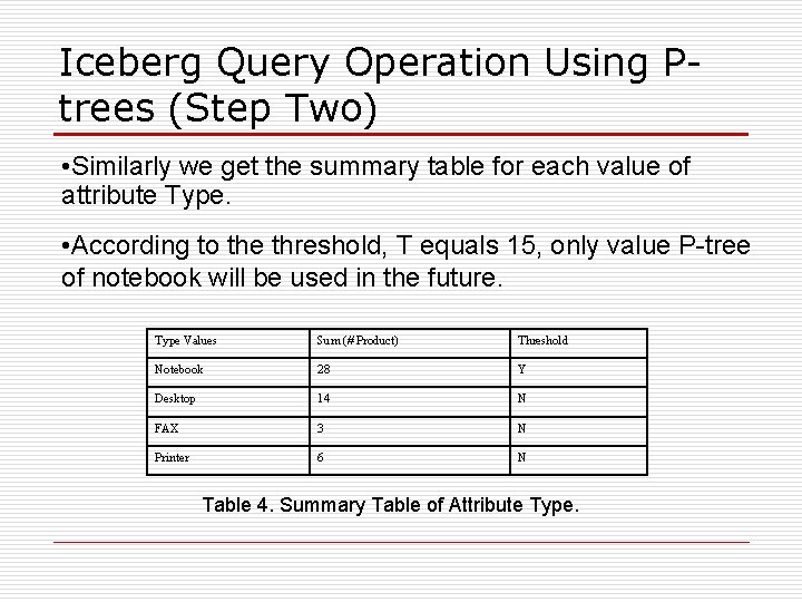
Iceberg Query Operation Using Ptrees (Step Two) • Similarly we get the summary table for each value of attribute Type. • According to the threshold, T equals 15, only value P-tree of notebook will be used in the future. Type Values Sum (# Product) Threshold Notebook 28 Y Desktop 14 N FAX 3 N Printer 6 N Table 4. Summary Table of Attribute Type.

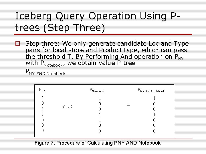
Iceberg Query Operation Using Ptrees (Step Three) o Step three: We only generate candidate Loc and Type pairs for local store and Product type, which can pass the threshold T. By Performing And operation on PNY with PNotebook, we obtain value P-tree PNY AND Notebook PNY 1 0 1 1 0 0 0 PNotebook AND 1 0 0 1 1 0 0 PNY AND Notebook = 1 0 0 0 Figure 7. Procedure of Calculating PNY AND Notebook

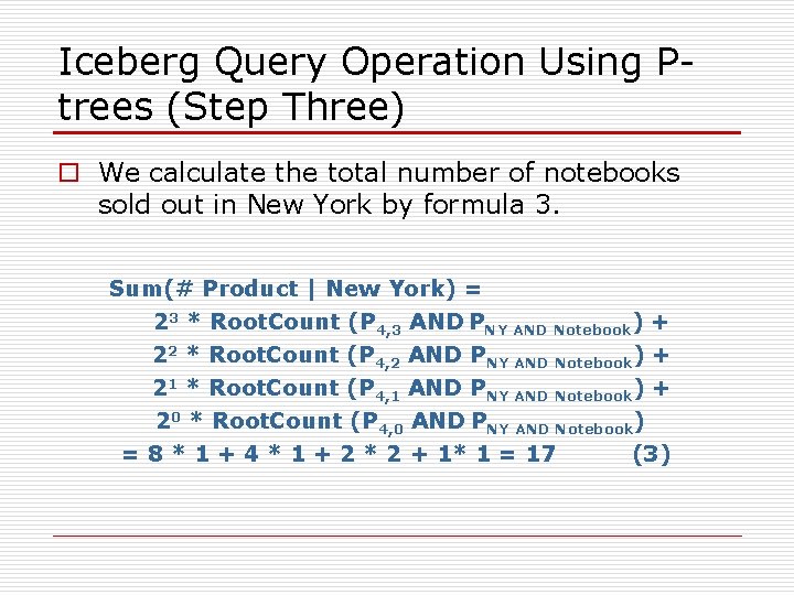
Iceberg Query Operation Using Ptrees (Step Three) o We calculate the total number of notebooks sold out in New York by formula 3. Sum(# Product | New York) = 23 * Root. Count (P 4, 3 AND PNY AND Notebook) + 22 * Root. Count (P 4, 2 AND PNY AND Notebook) + 21 * Root. Count (P 4, 1 AND PNY AND Notebook) + 20 * Root. Count (P 4, 0 AND PNY AND Notebook) = 8 * 1 + 4 * 1 + 2 * 2 + 1* 1 = 17 (3)

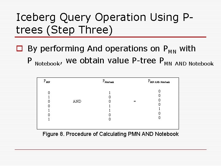
Iceberg Query Operation Using Ptrees (Step Three) o By performing And operations on PMN with P Notebook, we obtain value P-tree PMN AND Notebook PMN 0 1 0 1 PNotebook AND 1 0 0 1 1 0 0 PMN AND Notebook = 0 0 1 0 0 Figure 8. Procedure of Calculating PMN AND Notebook

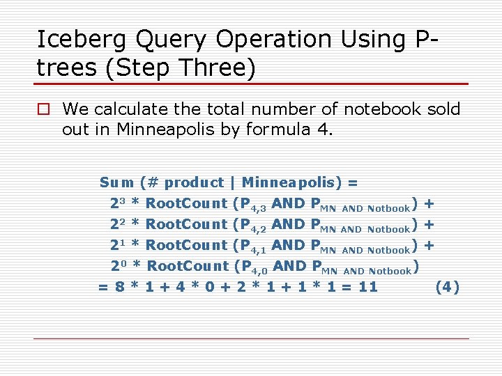
Iceberg Query Operation Using Ptrees (Step Three) o We calculate the total number of notebook sold out in Minneapolis by formula 4. Sum (# product | Minneapolis) = 23 * Root. Count (P 4, 3 AND PMN AND Notbook) + 22 * Root. Count (P 4, 2 AND PMN AND Notbook) + 21 * Root. Count (P 4, 1 AND PMN AND Notbook) + 20 * Root. Count (P 4, 0 AND PMN AND Notbook) = 8 * 1 + 4 * 0 + 2 * 1 + 1 * 1 = 11 (4)

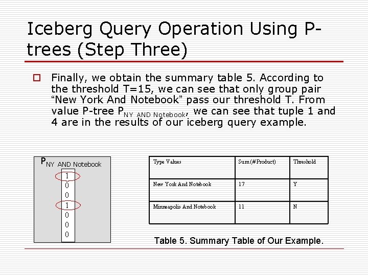
Iceberg Query Operation Using Ptrees (Step Three) o Finally, we obtain the summary table 5. According to the threshold T=15, we can see that only group pair “New York And Notebook” pass our threshold T. From value P-tree PNY AND Notebook, we can see that tuple 1 and 4 are in the results of our iceberg query example. PNY AND Notebook 1 0 0 0 Type Values Sum (# Product) Threshold New York And Notebook 17 Y Minneapolis And Notebook 11 N Table 5. Summary Table of Our Example.

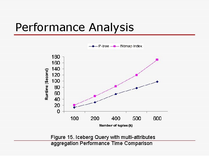
Performance Analysis Figure 15. Iceberg Query with multi-attributes aggregation Performance Time Comparison

Performance Analysis o Our experiments are implemented in the C++ language on a 1 GHz Pentium PC machine with 1 GB main memory running on Red Hat Linux. o In figure 15, we compare the running time of P -tree method and bitmap method on calculating multi-attribute iceberg query. In this case Ptrees are proved to be substantially faster.

Conclusion o we believe our study confirms that the P-tree approach is superior to the bitmap approach for aggregation of all types and multi-attribute iceberg queries. o It also proves that the advantages of basic P-tree representations of files are: n First, there is no need for redundant, auxiliary structures. n Second basic P-trees are good at calculating multiattribute aggregations, numeric value, and fair to all attributes.

Thank you !