Aggregate Demand Aggregate Supply Main macroeconomic model Aggregate

Aggregate Demand Aggregate Supply Main macroeconomic model

Aggregate Demand (AD) • What does “aggregate” mean? – Total What does “demand” mean ? – Quantity of good/services people are willing and able to purchase at different prices • Aggregate demand is the total spending on goods and services in a period of time at different price levels • Why do the following people need to know about AD?

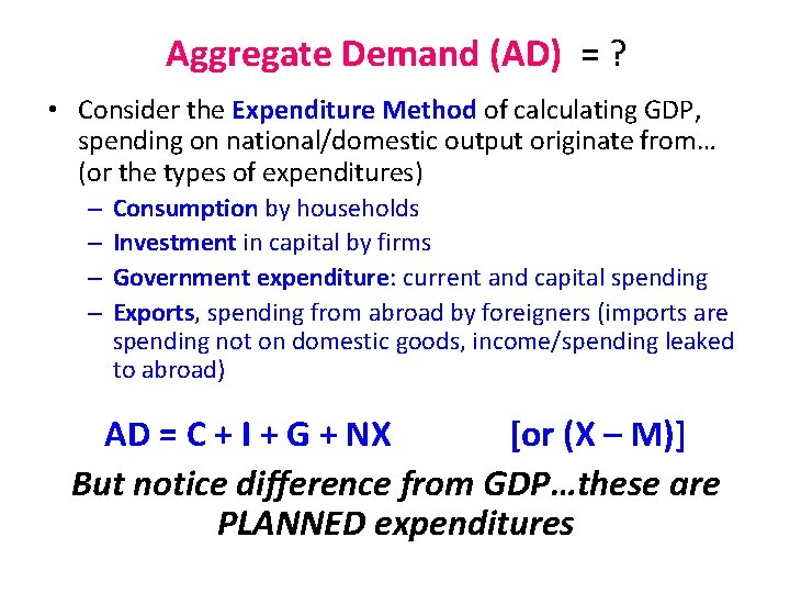
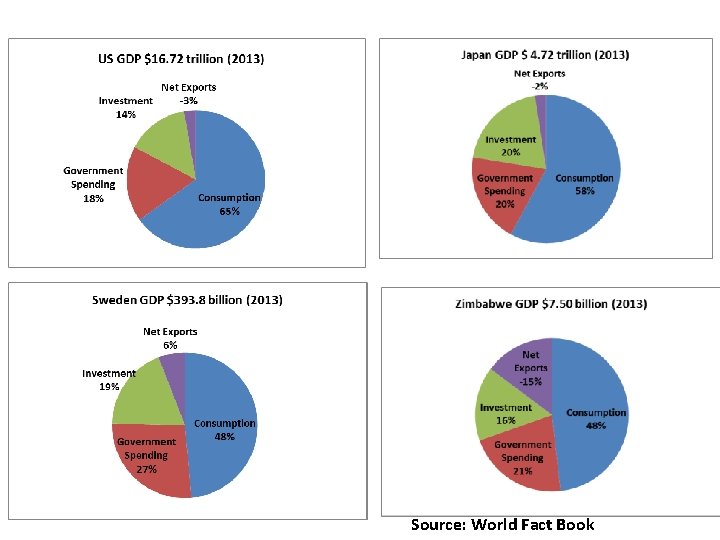
Aggregate Demand (AD) = ? • Consider the Expenditure Method of calculating GDP, spending on national/domestic output originate from… (or the types of expenditures) – – Consumption by households Investment in capital by firms Government expenditure: current and capital spending Exports, spending from abroad by foreigners (imports are spending not on domestic goods, income/spending leaked to abroad) AD = C + I + G + NX [or (X – M)] But notice difference from GDP…these are PLANNED expenditures

Source: World Fact Book

Modeling the Aggregate Demand • Economists use graphs and mathematical equations to explain, analyze, and forecast AD and the economic outcomes. • They will also use AD to predict the possible effects of different macroeconomic policies

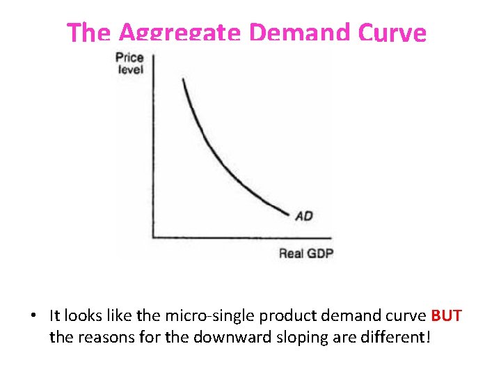
The Aggregate Demand Curve • It looks like the micro-single product demand curve BUT the reasons for the downward sloping are different!

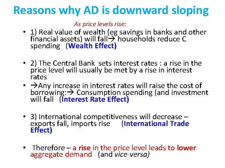
Reasons why AD is downward sloping As price levels rise: • 1) Real value of wealth (eg savings in banks and other financial assets) will fall households reduce C spending (Wealth Effect) • 2) The Central Bank sets interest rates : a rise in the price level will usually be met by a rise in interest rates • Any increase in interest rates will raise the cost of borrowing: Consumption spending (and investment will fall (Interest Rate Effect) • 3) International competitiveness will decrease – exports fall, imports rise (International Trade Effect) • Therefore – a rise in the price level leads to lower aggregate demand (and vice-versa)

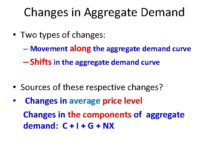
Changes in Aggregate Demand • Two types of changes: – Movement along the aggregate demand curve – Shifts in the aggregate demand curve • Sources of these respective changes? • Changes in average price level Changes in the components of aggregate demand: C + I + G + NX

The Determinants of the Components of Aggregate Demand - what factors shift the AD ? -

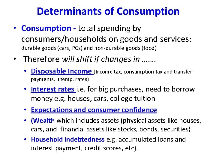
Determinants of Consumption • Consumption - total spending by consumers/households on goods and services: durable goods (cars, PCs) and non-durable goods (food) • Therefore will shift if changes in ……. • Disposable Income (Income tax, consumption tax and transfer payments, unemp. rates) • Interest rates i. e. for big purchases, need to borrow money e. g. houses, cars, college tuition • Expectations and consumer confidence • (Wealth which includes assets (physical assets like houses, cars, and financial assets like stocks, bonds, securities) • Household indebtedness e. g. accumulated loans and interest payment, credit scores, etc).

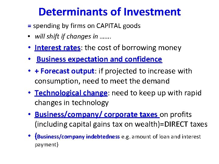
Determinants of Investment = spending by firms on CAPITAL goods • will shift if changes in ……. • Interest rates: the cost of borrowing money • Business expectation and confidence • + Forecast output: if projected to increase with consumption, need to meet the demand • Technological change: need to keep up with rapid changes in technology • Business/company/ corporate taxes on profits (including capital gains tax on wealth)=DIRECT taxes • (Business/company indebtedness e. g. amount of loan and interest payment)

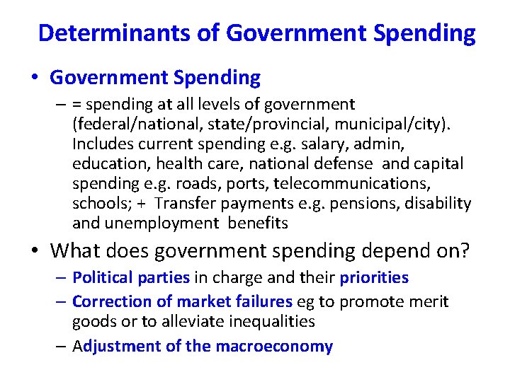
Determinants of Government Spending • Government Spending – = spending at all levels of government (federal/national, state/provincial, municipal/city). Includes current spending e. g. salary, admin, education, health care, national defense and capital spending e. g. roads, ports, telecommunications, schools; + Transfer payments e. g. pensions, disability and unemployment benefits • What does government spending depend on? – Political parties in charge and their priorities – Correction of market failures eg to promote merit goods or to alleviate inequalities – Adjustment of the macroeconomy

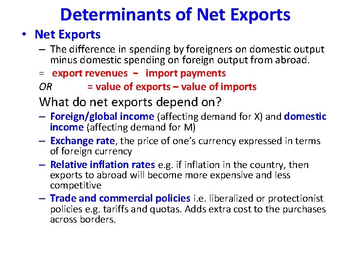
Determinants of Net Exports • Net Exports – The difference in spending by foreigners on domestic output minus domestic spending on foreign output from abroad. = export revenues − import payments OR = value of exports – value of imports What do net exports depend on? – Foreign/global income (affecting demand for X) and domestic income (affecting demand for M) – Exchange rate, the price of one’s currency expressed in terms of foreign currency – Relative inflation rates e. g. if inflation in the country, then exports to abroad will become more expensive and less competitive – Trade and commercial policies i. e. liberalized or protectionist policies e. g. tariffs and quotas. Adds extra cost to the purchases across borders.

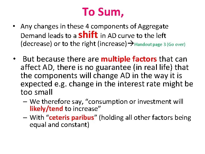
To Sum, • Any changes in these 4 components of Aggregate Demand leads to a shift in AD curve to the left (decrease) or to the right (increase) Handout page 3 (Go over) • But because there are multiple factors that can affect AD, there is no guarantee (in real life) that the components will change AD in the way it is expected e. g. change in the interest rate might be too small – We therefore say, “consumption or investment will likely/tend to increase” – With “ceteris paribus” (holding all other factors being equal and constant)

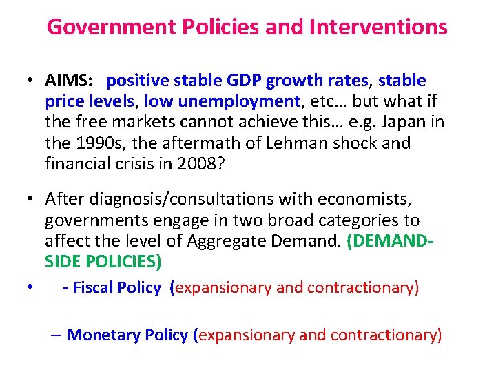
Government Policies and Interventions • AIMS: positive stable GDP growth rates, stable price levels, low unemployment, etc… but what if the free markets cannot achieve this… e. g. Japan in the 1990 s, the aftermath of Lehman shock and financial crisis in 2008? • After diagnosis/consultations with economists, governments engage in two broad categories to affect the level of Aggregate Demand. (DEMANDSIDE POLICIES) • - Fiscal Policy (expansionary and contractionary) – Monetary Policy (expansionary and contractionary)

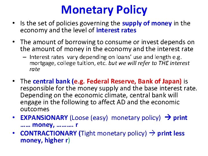
Monetary Policy • Is the set of policies governing the supply of money in the economy and the level of interest rates • The amount of borrowing to consume or invest depends on the amount of money in the economy and the interest rate – Interest rates vary depending on loans’ use and length e. g. mortgage, college tuition, etc. but we will refer to THE interest rate • The central bank (e. g. Federal Reserve, Bank of Japan) is responsible for the money supply and the base interest rate. Depending on the economic climate, central bank will engage in the following to affect AD and the economic outcomes • EXPANSIONARY (Loose (easy) monetary policy) print …… money, ………. r • CONTRACTIONARY (Tight monetary policy) print less money, higher r)

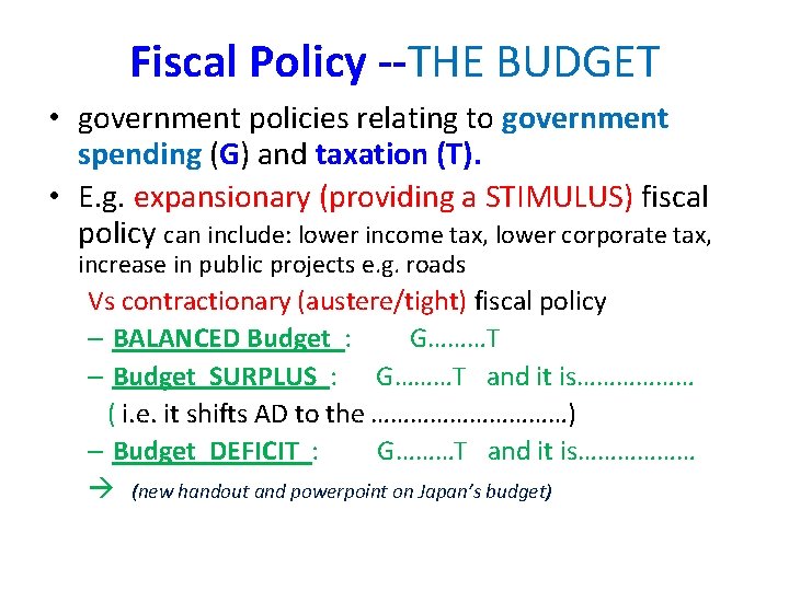
Fiscal Policy --THE BUDGET • government policies relating to government spending (G) and taxation (T). • E. g. expansionary (providing a STIMULUS) fiscal policy can include: lower income tax, lower corporate tax, increase in public projects e. g. roads Vs contractionary (austere/tight) fiscal policy – BALANCED Budget : G………T – Budget SURPLUS : G………T and it is……………… ( i. e. it shifts AD to the ……………) – Budget DEFICIT : G………T and it is……………… (new handout and powerpoint on Japan’s budget)

Aggregate Supply • NOTICE: several different types of AS curve! (though only one type of AD curve) Group III

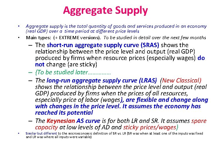
Aggregate Supply • • • Aggregate supply is the total quantity of goods and services produced in an economy (real GDP) over a time period at different price levels Main types: (+ EXTREME versions). To be studied in detail over the next few months – The short-run aggregate supply curve (SRAS) shows the relationship between the price level and output (real GDP) produced by firms when resource prices (especially wages) do not change (are sticky) – {To be studied later…………… – The long-run aggregate supply curve (LRAS) (New Classical) shows the relationship between the price level and output (real GDP) produced by firms when the prices of all resources, especially price of labor (wages), are flexible and change along with changes in the price level. It assumes the economy has reached its potential – The Keynesian AS curve is for both LR and SR. It assumes spare capacity at low levels of AD and sticky prices/wages} Similar but different to the microeconomic definition of SR vs. LR (SR was when at least one of the inputs was fixed and LR was where all inputs were variable)

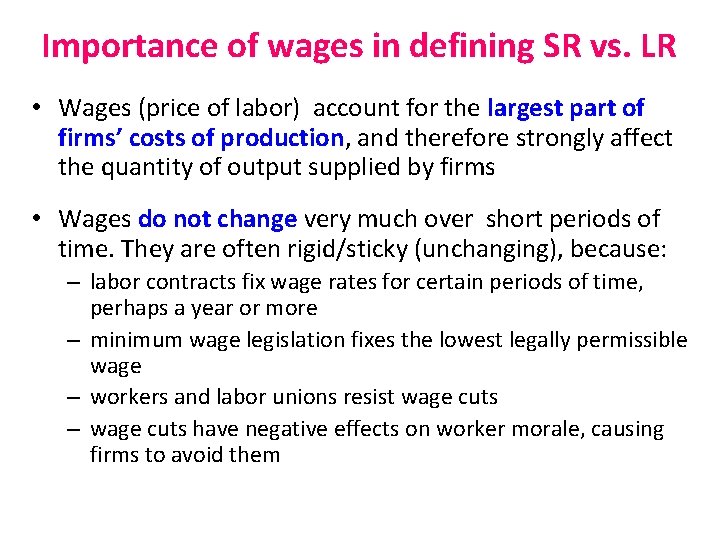
Importance of wages in defining SR vs. LR • Wages (price of labor) account for the largest part of firms’ costs of production, and therefore strongly affect the quantity of output supplied by firms • Wages do not change very much over short periods of time. They are often rigid/sticky (unchanging), because: – labor contracts fix wage rates for certain periods of time, perhaps a year or more – minimum wage legislation fixes the lowest legally permissible wage – workers and labor unions resist wage cuts – wage cuts have negative effects on worker morale, causing firms to avoid them

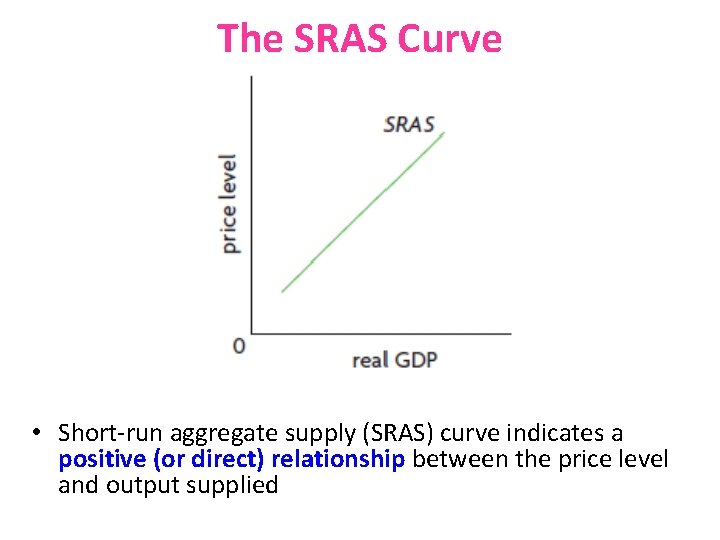
The SRAS Curve • Short-run aggregate supply (SRAS) curve indicates a positive (or direct) relationship between the price level and output supplied

Why is SRAS curve upward-sloping? • Explanation is based on firms’ profitability: – when there is an increase in the price level, this means that FINAL output prices have increased; but with unchanging resource prices (since the economy is in the short run), firms’ profits increase – As production becomes more profitable, firms increase the quantity of output produced

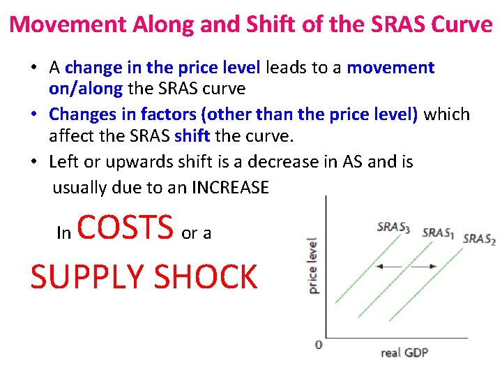
Movement Along and Shift of the SRAS Curve • A change in the price level leads to a movement on/along the SRAS curve • Changes in factors (other than the price level) which affect the SRAS shift the curve. • Left or upwards shift is a decrease in AS and is usually due to an INCREASE COSTS or a SUPPLY SHOCK In

Factors that Shift the SRAS: details ( group III. Thurs) • Firms’ COSTS (ie average or costs per unit) of production: – Changes in wages: for example due to changes in minimum wage legislation or labor union bargaining with employers. – Changes in resource prices: such as the price of oil, equipment, capital goods, land inputs, etc. – Changes in productivity (eg due to tech): higher productivity …………. costs – Changes in business taxes on profits (corporate taxes) are costs of production – Changes in subsidies. If they increase, the SRAS curve shifts to the right • Supply shocks: – War or violent conflict, unfavorable weather, sudden rise in oil prices (“oil shock”) can all lead to a leftward shift in the SRAS curve – Good weather or new technologies can lead to a rightward shift in the SRAS

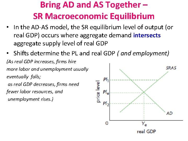
Bring AD and AS Together – SR Macroeconomic Equilibrium • In the AD-AS model, the SR equilibrium level of output (or real GDP) occurs where aggregate demand intersects aggregate supply level of real GDP • Shifts determine the PL and real GDP ( and employment) (As real GDP increases, firms hire more labor and unemployment usually eventually falls; as real GDP decreases, firms need fewer labor resources, and unemployment rises. )

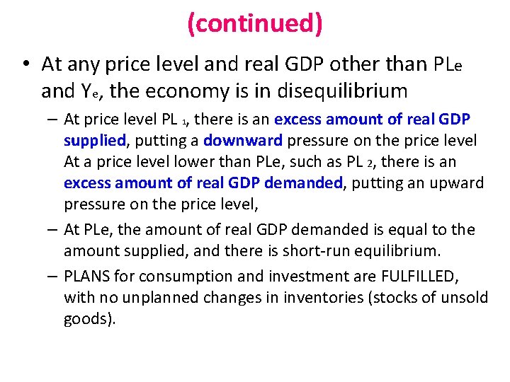
(continued) • At any price level and real GDP other than PLe and Ye, the economy is in disequilibrium – At price level PL 1, there is an excess amount of real GDP supplied, putting a downward pressure on the price level At a price level lower than PLe, such as PL 2, there is an excess amount of real GDP demanded, putting an upward pressure on the price level, – At PLe, the amount of real GDP demanded is equal to the amount supplied, and there is short-run equilibrium. – PLANS for consumption and investment are FULFILLED, with no unplanned changes in inventories (stocks of unsold goods).

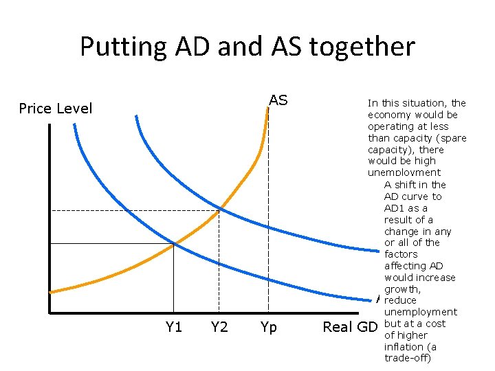
Putting AD and AS together AS Price Level Y 1 Y 2 Yp Real In this situation, the economy would be operating at less than capacity (spare capacity), there would be high unemployment A shift in the AD curve to AD 1 as a result of a change in any or all of the AD 1 factors affecting AD would increase growth, AD reduce unemployment GDPbut at a cost of higher inflation (a trade-off)

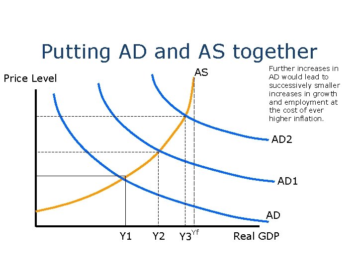
Putting AD and AS together AS Price Level Further increases in AD would lead to successively smaller increases in growth and employment at the cost of ever higher inflation. AD 2 AD 1 AD Y 1 Y 2 Yf Y 3 Real GDP

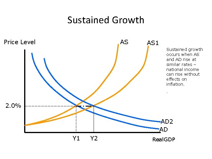
Sustained Growth Price Level AS AS 1 Sustained growth occurs when AS and AD rise at similar rates – national income can rise without effects on inflation. . 2. 0% AD 2 AD Y 1 Y 2 Real. GDP

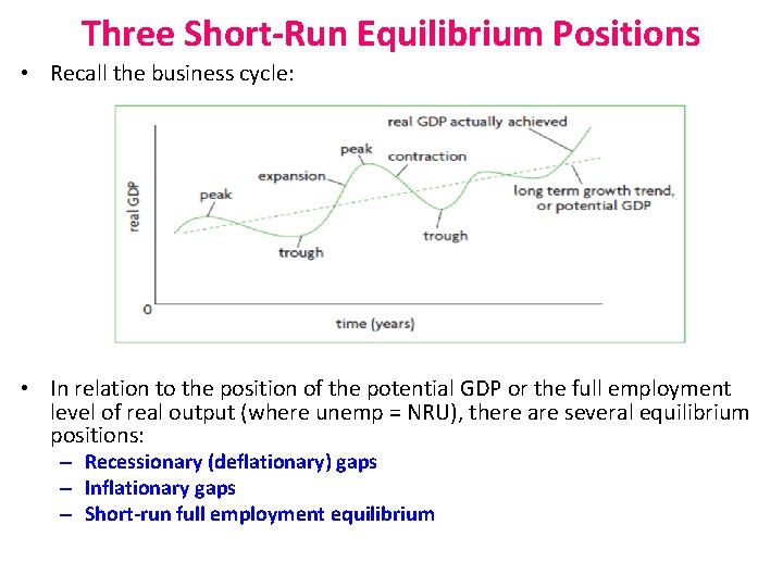
Three Short-Run Equilibrium Positions • Recall the business cycle: • In relation to the position of the potential GDP or the full employment level of real output (where unemp = NRU), there are several equilibrium positions: – Recessionary (deflationary) gaps – Inflationary gaps – Short-run full employment equilibrium

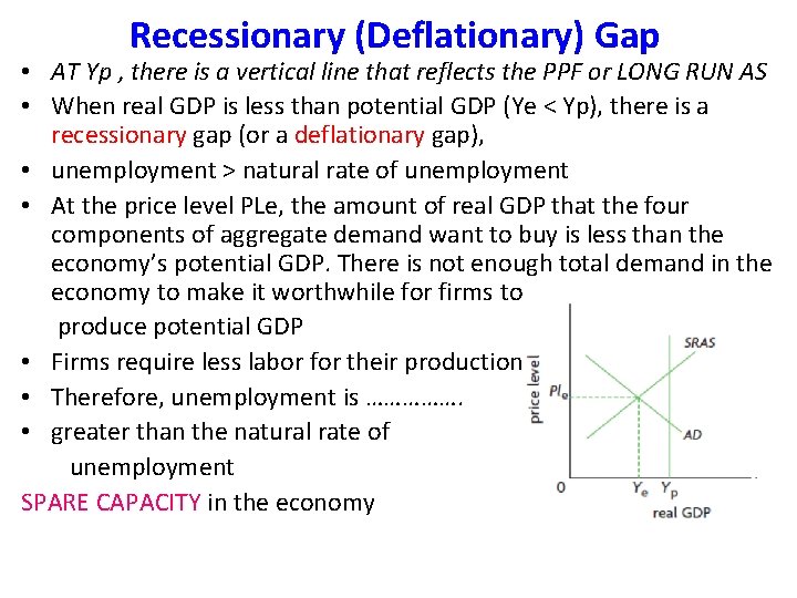
Recessionary (Deflationary) Gap • AT Yp , there is a vertical line that reflects the PPF or LONG RUN AS • When real GDP is less than potential GDP (Ye < Yp), there is a recessionary gap (or a deflationary gap), • unemployment > natural rate of unemployment • At the price level PLe, the amount of real GDP that the four components of aggregate demand want to buy is less than the economy’s potential GDP. There is not enough total demand in the economy to make it worthwhile for firms to produce potential GDP • Firms require less labor for their production; • Therefore, unemployment is ……………. • greater than the natural rate of unemployment SPARE CAPACITY in the economy

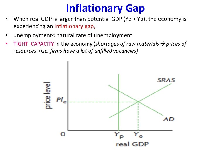
Inflationary Gap • When real GDP is larger than potential GDP (Ye > Yp), the economy is experiencing an inflationary gap, • unemployment< natural rate of unemployment • TIGHT CAPACITY in the economy (shortages of raw materials prices of resources rise, firms have a lot of unfilled vacancies)

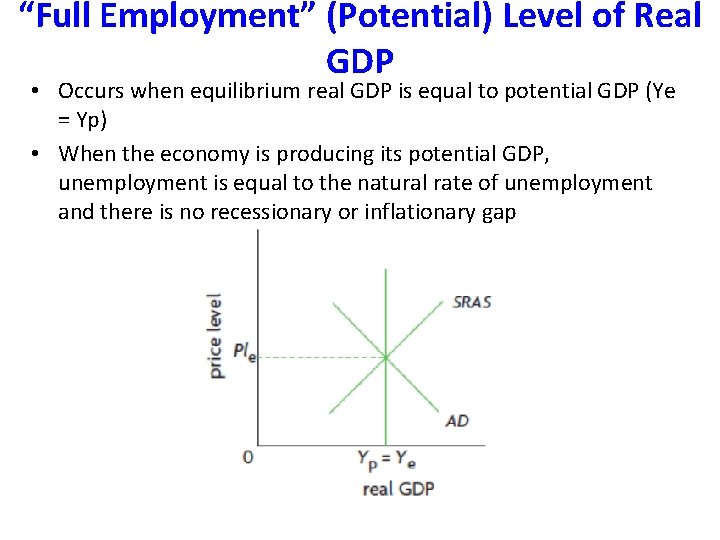
“Full Employment” (Potential) Level of Real GDP • Occurs when equilibrium real GDP is equal to potential GDP (Ye = Yp) • When the economy is producing its potential GDP, unemployment is equal to the natural rate of unemployment and there is no recessionary or inflationary gap

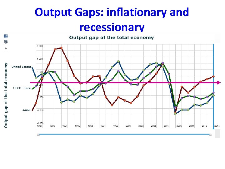
Output Gaps: inflationary and recessionary

The Significance of this Analysis? • Potential GDP demonstrates the productive capacity of the economy • If equilibrium GDP ≠ potential GDP, government can consider whether and to what extent to intervene in the economy • Governments need to know and forecast (using computer models) the economy’s limits • The Federal Reserve, Bank of Japan, International Monetary Fund (IMF) are therefore always making computer simulations of potential and equilibrium GDP using unemp. data and other measures