Aggregate Demand Aggregate Supply and Fiscal Policy AP

Aggregate Demand, Aggregate Supply and Fiscal Policy AP Economics Chapters 11 -12

BACKGROUND Classical Economic Theory • Market system operated at full employment • Temporary short periods of recession or inflation • Self correcting (P & Wages go up & down) • Say’s Law: “Supply creates its own demand” • Accepted view until 1930’s and the Great Depression

BACKGROUND Keynes “In the long run, we are all dead” Keynes believed ~ • Cycles were not short • Corrections were not automatic • Savings and investment weren’t coordinated • Prices and wages were not flexible downward GOV INTERVENTION WAS NEEDED

KEYNES • • • Fiscal Policy is government’s way to stabilize the economy Employment Act of 1946 - power to Congress Tools to use: taxing and spending Expansionary F. P. – Decrease taxes &/or increase spending (Recession) Contractionary F. P. – Increase taxes &/or decrease spending (Inflation)

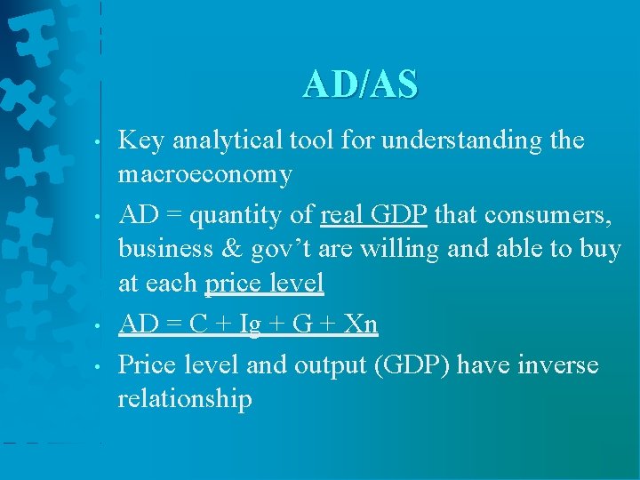
AD/AS • • Key analytical tool for understanding the macroeconomy AD = quantity of real GDP that consumers, business & gov’t are willing and able to buy at each price level AD = C + Ig + G + Xn Price level and output (GDP) have inverse relationship

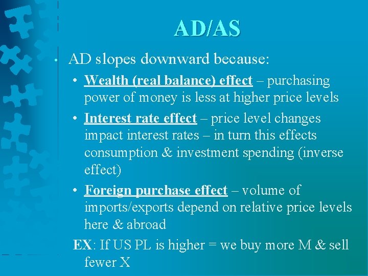
AD/AS • AD slopes downward because: • Wealth (real balance) effect – purchasing power of money is less at higher price levels • Interest rate effect – price level changes impact interest rates – in turn this effects consumption & investment spending (inverse effect) • Foreign purchase effect – volume of imports/exports depend on relative price levels here & abroad EX: If US PL is higher = we buy more M & sell fewer X

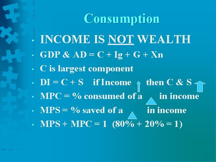
Consumption • • INCOME IS NOT WEALTH GDP & AD = C + Ig + G + Xn C is largest component DI = C + S if Income then C & S MPC = % consumed of a in income MPS = % saved of a in income MPS + MPC = 1 (80% + 20% = 1)

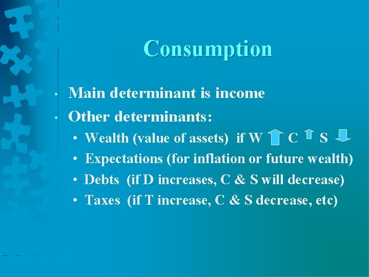
Consumption • • Main determinant is income Other determinants: • • Wealth (value of assets) if W C S Expectations (for inflation or future wealth) Debts (if D increases, C & S will decrease) Taxes (if T increase, C & S decrease, etc)

Investment • • Savings = Investment is: • • Business spending for capital stock Most volatile component of AD/GDP Assumed to require a loan Decisions are based on marginal cost (interest) vs. marginal benefits (expected rate of return)

Investment Economic profit/cost = Rate of return EX: $100 profit divided by $1000 cost = 10% • Interest must be less than rate of return to justify investment • Investment determinants: • • • Interest rate Costs of capital & operating costs Taxes Technology Excess capacity (inventories)

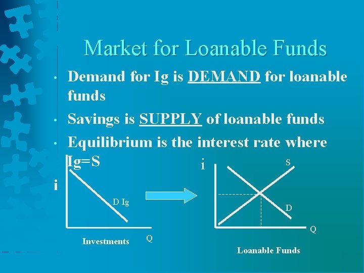
Market for Loanable Funds • • • Demand for Ig is DEMAND for loanable funds Savings is SUPPLY of loanable funds Equilibrium is the interest rate where S Ig=S i i D Ig Investments D Q Q Loanable Funds

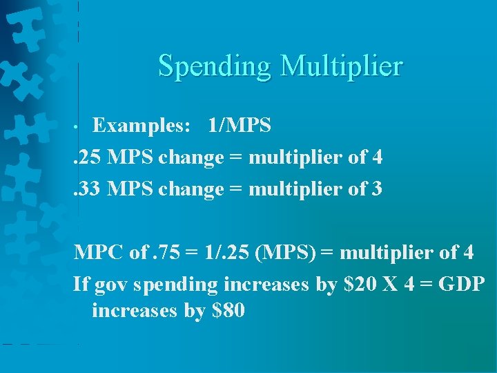
Spending Multiplier • • • Change to any component of AD (C + Ig + G + Xn) has a “ripple effect” Results in a multiplied effect on GDP Important as a small change in spending leads to a large change in GDP Assumes that change occurs first to Ig Calculated by: 1 or 1 MPS 1 - MPC

Spending Multiplier Examples: 1/MPS. 25 MPS change = multiplier of 4. 33 MPS change = multiplier of 3 • MPC of. 75 = 1/. 25 (MPS) = multiplier of 4 If gov spending increases by $20 X 4 = GDP increases by $80

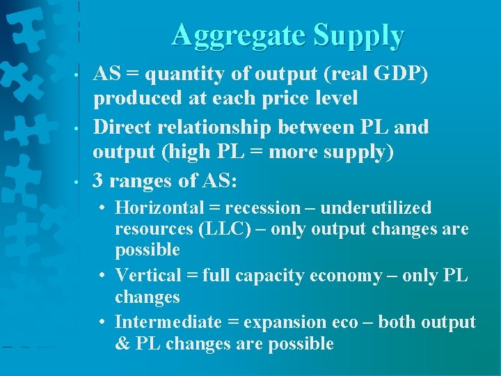
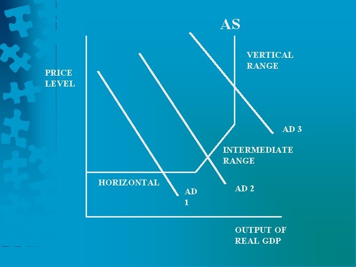
Aggregate Supply • • • AS = quantity of output (real GDP) produced at each price level Direct relationship between PL and output (high PL = more supply) 3 ranges of AS: • Horizontal = recession – underutilized resources (LLC) – only output changes are possible • Vertical = full capacity economy – only PL changes • Intermediate = expansion eco – both output & PL changes are possible

AS VERTICAL RANGE PRICE LEVEL AD 3 INTERMEDIATE RANGE HORIZONTAL AD 1 AD 2 OUTPUT OF REAL GDP

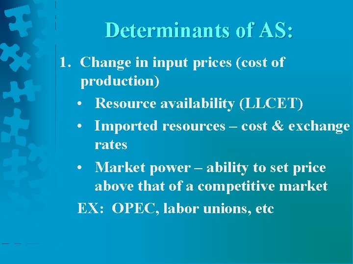
Determinants of AS: 1. Change in input prices (cost of production) • Resource availability (LLCET) • Imported resources – cost & exchange rates • Market power – ability to set price above that of a competitive market EX: OPEC, labor unions, etc

Determinants of AS: 2. Change in productivity – increase means can produce more with same resources EX: more productivity = increase AS 3. Change in legal-institution environment Taxes (sales, excise, payroll) = increase costs of production (AS decreases) Subsidies – gov’t payment = lowers costs (AS increases) Gov’t regulations = costs more to comply so AS decreases

Other Details: • Multiplier effect is: • greatest in the horizontal AS range (much ability to increase GDP) • less in the intermediate range (increasing PL leads to inflation) • None in the vertical range ( GDP does not change – only price level)

Other Details: • RATCHET EFFECT (or “sticky wages”) • Prices don’t always go down when AD shifts left due to: wage contracts, worker morale, minimum wage laws, “menu costs” – costs to change prices up & down frequently & fear of “price wars” with competition. SHORT RUN – period when wages & other costs are FIXED (suppliers need time to adjust to change in AD/AS) LONG RUN – period when suppliers can make adjustments in LLC due to a change in AD/AS

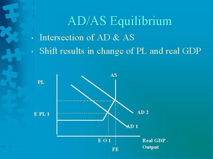
AD/AS Equilibrium • • Intersection of AD & AS Shift results in change of PL and real GDP AS PL AD 2 E PL 1 AD 1 EO 1 FE Real GDP Output

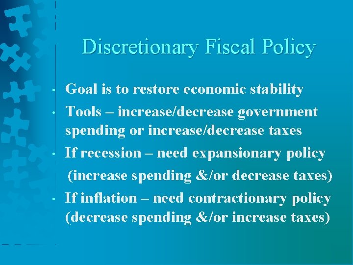
Discretionary Fiscal Policy • • Goal is to restore economic stability Tools – increase/decrease government spending or increase/decrease taxes If recession – need expansionary policy (increase spending &/or decrease taxes) If inflation – need contractionary policy (decrease spending &/or increase taxes)

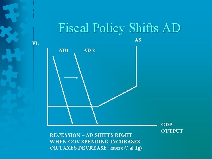
Fiscal Policy Shifts AD AS PL AD 1 AD 2 RECESSION – AD SHIFTS RIGHT WHEN GOV SPENDING INCREASES OR TAXES DECREASE (more C & Ig) GDP OUTPUT

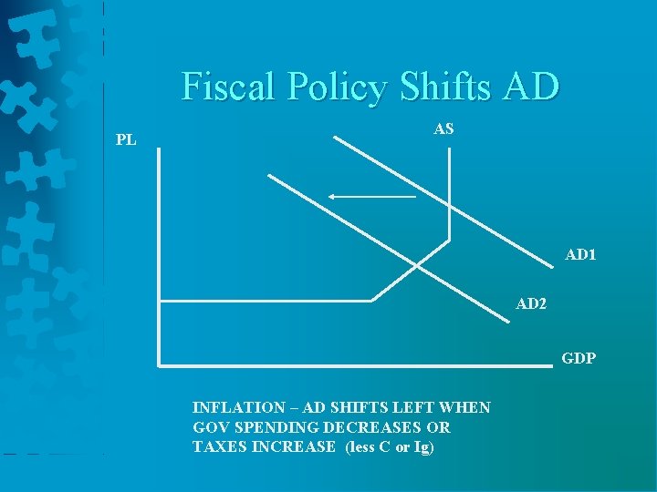
Fiscal Policy Shifts AD PL AS AD 1 AD 2 GDP INFLATION – AD SHIFTS LEFT WHEN GOV SPENDING DECREASES OR TAXES INCREASE (less C or Ig)

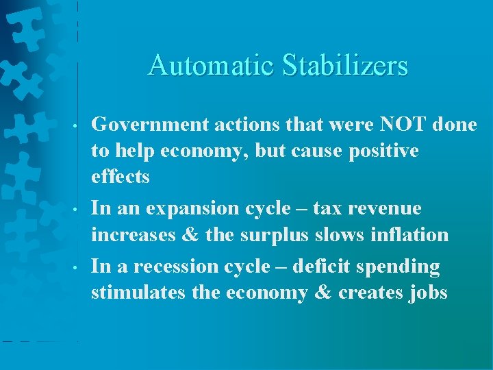
Automatic Stabilizers • • • Government actions that were NOT done to help economy, but cause positive effects In an expansion cycle – tax revenue increases & the surplus slows inflation In a recession cycle – deficit spending stimulates the economy & creates jobs

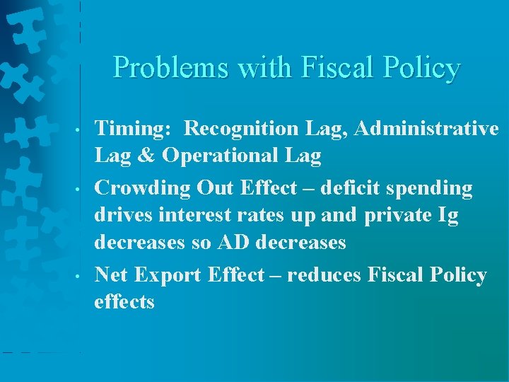
Problems with Fiscal Policy • • • Timing: Recognition Lag, Administrative Lag & Operational Lag Crowding Out Effect – deficit spending drives interest rates up and private Ig decreases so AD decreases Net Export Effect – reduces Fiscal Policy effects

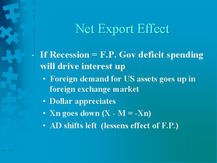
Net Export Effect • If Recession = F. P. Gov deficit spending will drive interest up • Foreign demand for US assets goes up in foreign exchange market • Dollar appreciates • Xn goes down (X - M = -Xn) • AD shifts left (lessens effect of F. P. )

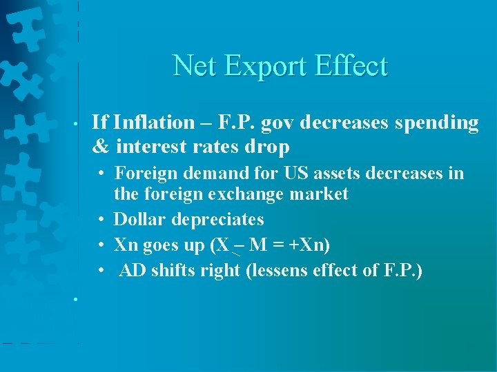
Net Export Effect • If Inflation – F. P. gov decreases spending & interest rates drop • Foreign demand for US assets decreases in the foreign exchange market • Dollar depreciates • Xn goes up (X – M = +Xn) • AD shifts right (lessens effect of F. P. ) •

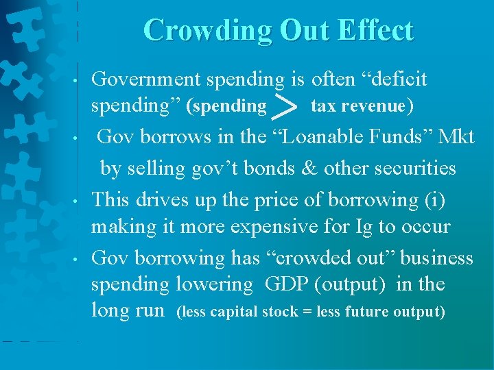
Crowding Out Effect • • Government spending is often “deficit spending” (spending tax revenue) Gov borrows in the “Loanable Funds” Mkt by selling gov’t bonds & other securities This drives up the price of borrowing (i) making it more expensive for Ig to occur Gov borrowing has “crowded out” business spending lowering GDP (output) in the long run (less capital stock = less future output)

Supply Side Fiscal Policy • Theory to cut taxes to increase AS • Encourages savings to give businesses an incentive to expand investments • Lower income taxes encourage workers to work more & earn more • Entrepreneurs are more willing to take risks when they get more rewards

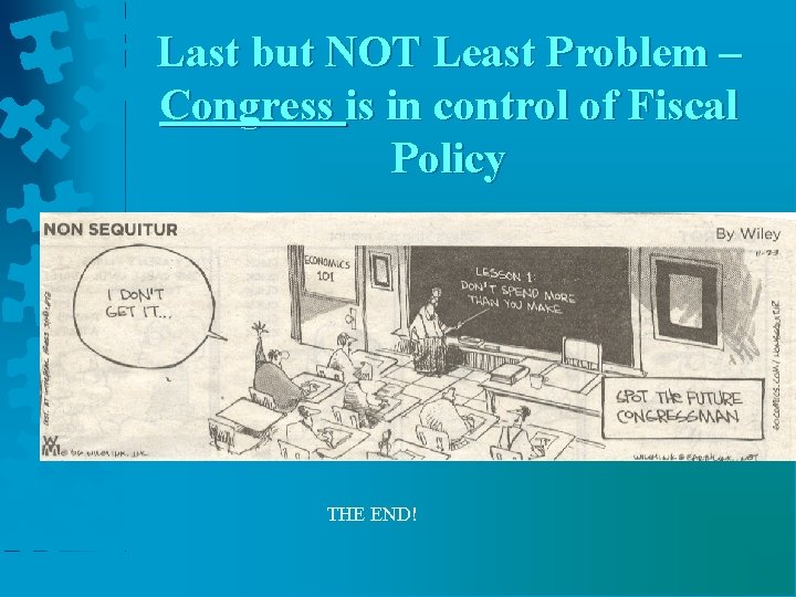
Last but NOT Least Problem – Congress is in control of Fiscal Policy THE END!