AGATA Data Processing Dino Bazzacco INFN Padova Topics

AGATA Data Processing Dino Bazzacco INFN Padova

Topics • • • General structure of data acquisition Data processing model == data analysis model Narval (ADA/C/C++) and actors emulators Data flow adf Survey of actors • Hands on

AGATA detectors 80 mm 90 mm Volume ~370 cc Weight ~2 kg (shapes are volume-equalized to 1%) 6 x 6 segmented cathode Cold FET for all signals Energy resolution Core: 2. 35 ke. V Segments: 2. 10 ke. V (FWHM @ 1332 ke. V) A. Wiens et al. NIM A 618 (2010) 223 D. Lersch et al. NIM A 640(2011) 133 38 high-resolution signals / detector AGATA capsules Manufactured by Canberra France AGATA Triple/Double Cryostat Manufactured by CTT

Structure of Electronics and DAQ GL Trigger Detector preamp. Digitisers Up to 180 detectors Pre. Processing & PSA Ancillary Clock 100 MHz T-Stamp Analogue Core + 36 seg. Preprocessing Electronics Ancillary Synchronous Event Builder Tracking Control, Storage… Buffered Other detectors 1. interface to GTS via mezzanine 2. merge time-stamped data into event builder (merger)

GTS : the system coordinator All detectors operated on the same 100 MHz clock Downwards Upwards Downwards 100 MHz clock + 48 bit Timestamp (updated every 16 clock cycles) trigger requests, consisting of address (8 bit) and timestamp (16 bit) max request rate 10 MHz total, 1 MHz/detector validations/rejections, consisting of request + event number (24 bit) Up to 256 requesters. Present implementation limited to 40 M. Bellato , Agata Week Darmstadt - 6 -9 September 2011

Architecture of the system • Local Level : where the individual detectors don’t know of each other. – Electronics and computing follow a model with minimum coupling among the individual detectors, which are operated independently as long as possible – Electronics is almost completely digital, operated on the same 100 MHz clock – Data processing (in the electronics and in the front-end computers) is the same for all detectors and proceeds in parallel – Every chunk of produced data is tagged with a 48 bit number (time stamp) giving the absolute time (with a precision of 10 ns) since the last hard-reset of the system roll around takes place every 32. 5 days. • Global Level : where the detectors do know of each other – By means of the real time trigger, which reduces the data rate by selecting the class of interesting events – Via the event builder and merger that assemble the event fragments (including the ancillaries) into complete events that are further processed – In the Tracking and in the Physical analysis stages v The fact that 3 (and 2 at GSI) crystals are packed in one cluster does not produce correlations in their data; only seen in the name of the detectors: v [1 -5][RGB] at LNL v [00 -14][ABC] at GSI and GANIL 2 G where 2 refers to the 2 nd cluster produced 12 B where 12 is the “hole” in the frame

00 A 00 B 00 C 01 A 01 B 01 C…. PSA Hits Auxiliary Digitizer+Pre. Proc or raw data file Producer VME or raw data file Ndets Crystal. Producer (Save original data) reading psa_xxx. adf Ndets Event. Builder Ancillary. Producer Event. Merger Ancillary. Filter Preprocessing. Filter PSAFilter Post. PSAFilter global actions and Tracking. Filter Consumer Save PSA output Save tracked output should be split in two actors

Narval Topology at LNL 5 ATC + 1 Ancillary Produced by the run control GUI Krakow at LNL

Data processing and replay • Offline = Online • A series of programs organized in the style of Narval actors • Director of the actors – Online : Narval – Offline : Narval or narval emulator(s) • Depending on the available computing resources • Single computer or Farm with distributed processing • The system is complex and “difficult” to manage – Very large number of channels Number. Of. Crystals*38 LNL 570 GSI 836 GANIL >1500 – No chance to take care of them individually – Rely on automatic procedures – Hope that the system is stable – Result depends on average performance • Need GUIs, Histogram Viewers and scripts to manage the work • Processing/Analysis model developed with contributions of several people – Xavier Grave, Olivier Stezowski and their groups for the architecture and the basic tools – Joa Ljungvall, Daniele Mengoni, Enrico Calore, Francesco Recchia – The users and their feedback

Emulator(s) • femul – Originally intended to help developing and debugging the user libraries which is very hard to do in a distributed processing environment like Narval. – Gradually developed as a full emulation of the Narval framework with the limitation of being a single process running a specific machine (threads used to distribute the work on the available cores). – Configuration (detectors, actors, . . ) specified by a “topology” file – Generation of configuration parameters vie gen_conf. py • Gamma. Ware and Watchers – Don’t know well its present status but this package is possibly more suitable for specific tasks and test, instead of inserting everything in an actor that is going to be used in the DAQ

Use of actors, managed by the framework (Narval or femul) • Creation – process_config and object creation … • process_initialise – Read parameters from conf. Path/Actor. conf (e. g. Conf/3 R/PSAFilter. conf ) – Generate configuration-dependent internal objects, open data files • process_start (Important for Producers/Consumers) • process_block (or adf: : Process. Block) – where the actual work is done the event loop • process_stop (Important for Producers/Consumers) • Destruction – Save spectra and close files • A fair amount of repeated code (boilerplate) saved by inheriting from proper base classes (Narval. Interface, Narval. Producer, Narval. Filter, Narval. Consumer provided by the adf library. • The C Narval API (and its C++ binding in the adf library) contain other lessused/less-useful functions

Olivier Stezowski

Olivier Stezowski

Olivier Stezowski

Structure of analysis directories • The directory where you produce your data ( e. g. /agatadisks/data/2011_week 41/z. Current. Narval. Data. Dir) contain some standard sub-directories – Conf configuration of actors, calibrations, . . . for each detector (e. g. @ LNL) 1 R 1 G 1 B 2 R. . . 5 B Ancillary Global with minimal differences between online and offline – Data data and spectra produced during the experiment 1 R 1 G 1 B 2 R. . . 5 B Ancillary Global Online writes data here Offline replay takes data from here – Out data and spectra produced during data replay 1 R 1 G 1 B 2 R. . . 5 B Ancillary Global Offline writes data here Conf, Data and Out are often symbolic links to actual directories

Typical configuration directories Conf/12 A • • • Crystal. Producer. conf Crystal. Producer. ATCA. conf Preprocessing. Filter. PSA. conf PSAFilter. conf Post. PSAFilter. conf xdir_1325 -1340. cal xinv_1325 -1340. cal Basic. AFC. conf Basic. AFP. conf Conf/Global • • • Event. Builder. conf Event. Merger. conf Tracking. Filter. conf Crystal. Position. Look. Up. Table Basic. AFC. conf

Binary spectra • Simple C-style multidimensional (max 6) arrays written mostly in binary format • For historical reasons the format is not recorded in the file. • Often written as part of the file name: – Prod__4 -38 -32768 -UI__Ampli. spec Is a file dump of an array defined as unsigned integer Ampli[4][38][32768] containing 4*38 = 152 spectra of 32768 channels – No difference between spectra and matrices; the type is only an hint to how to interpret them • The viewers Tk. T and Mat can decode and interpret the format. The user can always override the program. • Other programs (e. g. Recal. Energy) can interpret the spectrum length and type but the user has to specify the number of spectra to act upon.

Some Useful programs • Tk. T spectrum viewer (& al) tailored to composite detectors – A nightmare concerning programming-style, but contains ~all I need(ed) to analyze AGATA data. Virtually no documentation. • Recal. Energy – Analysis of spectra looking for peaks • x. Talk. Sort x. Talk. Invert (x. Talk. Make Sort. Capsule) – Sort and analysis of Agata events without traces • Sort. FFT – Fourier spectrum from “Long Traces” • Sort. Psa. Hits – Sort of PSA hits (special format) to determine neutron damage correction parameters • gen_conf. py – Unified procedure to produce configuration files for all actors • solve. TT. py – Optimize time alignment of “equal” detectors

Local Actors • Producers – Crystal. Producer • • • Filters Readout of electronics, or get raw data from file Local event builder Save original data to be able to replay experiment Raw projections – Preprocessing. Filter. PSA • • • Energy calibrations Retrigger and Time calibration Cross talk correction Amplitude calibration and time alignment of traces Improved pile-up rejection – PSAFilter. Grid. Search • Decomposition of calibrated experimental traces by comparison with a calculated signal basis • In principle more than one algorithm available but only one used in practice. – Post. PSAFilter • Neutron deficit corrections • Recalibrations of energy and time • Smearing of positions • Consumer – Save PSA hits for “Global Level”-only processing

Global Actors • Event Builder – Essentially a producer with multiple inputs – Assemble event fragments from Ge detectors (Builder) and Auxiliary detectors (Merger) • Filters – Tracking. Filter • • Global histograms (time, energy …) Grouping and further filtering Format data as needed by the specific Tracking Filter Histograms of tracked gammas • Consumer – Write tracked data

Crystal. Producer • Reads the data from: – The PCI express driver connected to the ATCA electronics – Raw data files (event_mezzdata. bdat) for the offline • Acts as a local event builder to check and merge the sub-events coming from the ATCA readout (or from the raw data file) – – For the online has to work in nonblocking-mode to avoid blocking the ACQ This feature was implemented with boost: : threads Damiano has now implemented the “select” and threads have been removed The local event builder and the management of the mezzanine data should be completely rewritten … • Can write the original data with the format of the ATCA electronics, and various other formats (e. g. only the energies for calibrations) • Prepares data: crystal frames, without using adf (version using adf exists, maybe slower) • Not much to do for the users both for Data Acquisition and Data Replay

What does it read and write • Raw event: data from 7 mezzanines hosted in two ATCA Carrier Boards • Mezzanine length (for 100 samples traces): 16+(8+100)*6 = 664 short (2 bytes) words • Event length: 7*664 = 9296 bytes • Local event builder to assemble data from 2 readout ports, according to mapping specified in Crystal. Producer. ATCA. conf contains the mapping • Write original data (event built, compressed 3. 6 k. B) – data files typically split after 1 M events ~ 3. 6 GB – event_mezzdata. cdat. 0000 event_mezzdata. cdat. 0001 … • Generate raw spectra for amplitudes and baselines • Format data into an data: crystal adf frame and send it to the data flow.

Raw data from EDAQ F 6 F 5 F 4 F 3 F 2 F 1 E 6 E 5 E 4 E 3 E 2 E 1 D 6 D 5 D 4 D 3 C 6 C 5 C 4 C 3 C 2 C 1 B 6 B 5 B 4 B 3 B 2 B 1 A 6 A 5 A 4 A 3 A 2 A 1 CC High Gain CC Low Gain D 2 D 1

Digitizers • 100 MS/s – max frequency correctly handled is 50 MHz (Nyquist) • 14 bits – Effective number of bits is ~12. 5 (SNR ~75 db) 2 cores (one board) and 36 segments (in 6 boards) Core 2 ranges 5, 20 Me. V nominal Segments taken either at high gain (5 Me. V) or at low gain (20 Me. V) The digitized samples are serialized and transmitted via optical fibre (1/channel) to the preprocessing electronics. Transmission rate is 2 Gbit/s on each of the 38 fibres. • Power consumption 240 W • Weight 35 kg • • • New digitizers and preprocessing electronics with same specs, much lower Power consumption, weight and cost have been developed (for AGATA and GALILEO) and are under test.

Range of digitizers 1 5 B 3 B 2 B 4 B 1 B 5 G 3 G 2 G 4 G 1 G 5 R 3 R 2 R 4 R 1 R Some cores and segments saturate below 3 Me. V on the high-gain range Gain in the digitizers should be reduced by ~30% test 5 atc_110603/run_000

Range of Digitizers Values derived from the energy calibration coefficients , with offsets adjusted to have the “zero”of preamp signals at ¼ of the conversion range Digitizer modified before the GANIL phase to better match the ranges of 6 and 20 Me. V

Range of digitizers 2 Operation at high counting rates 1 R CC high gain 1 R CC low gain 1 R B 1 (low gain) CC ~30 k. Hz segment B 1 ~7 k. Hz 1 ms

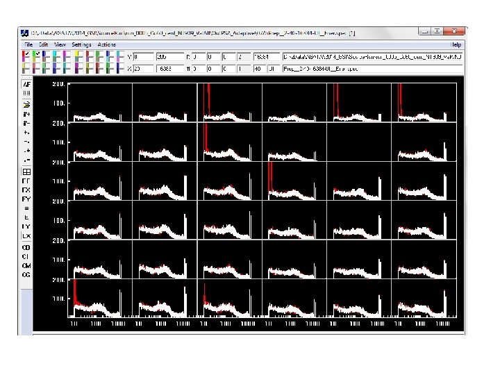
Prod__4 -38 -32768 -UI__Ampli. spec [1]-38 -32768 used for energy calibrations A 6 B 6 C 6 D 6 E 6 F 6 A 5 B 5 C 5 D 5 E 5 F 5 A 4 B 4 C 4 D 4 E 4 F 4 A 3 B 3 C 3 D 3 E 3 F 3 A 2 B 2 C 2 D 2 E 2 F 2 CC 1 Low Gain A 1 B 1 C 1 D 1 E 1 F 1 CC 0 High Gain

Prod__100000 -UI__Tst. Diff. spec ms

Preprocessing. Filter • Performs – Energy calibrations and cross talk corrections – Analysis of traces • • Calculation of T 0 from core (Digital CFD or linear fit of the first samples) Time calibrations and shifts Vertical normalization of traces Define the net-charge segments – Reformats the data as data: ccrystal frames – After Preprocessing: • energies are stored in units of ke. V • times are in units of samples (10 ns) (but time calibration parameters are in ns) • positions are given in mm, when they show up after the PSA

Calibrations • Energy – Gain-only, no offset coefficient needed because of the way the amplitude is generated in the preprocessing electronics. – Challenged by the Differential Non Linearity (DNL) of the ADC • Cross-talk – 36*36=1296 coefficients to correct capacitive coupling correlations between segments and core – Used also to recover up to one broken or missing segment per crystal • Time – Local 36 coefficients to alignment of segment to the core great influence on the performance of PSA – Global alignment of crystals and other detectors important to reduce random coincidences • Response function of the system – To match the PSA calculated signals to the real data • Neutron damage – Recover energy resolution of the segments using info from PSA.

Preprocessing. Filter. PSA. conf

Cross-Talk • Proportional – Affects energy spectra of multi-segment events – x. Talk. Sort … • Differential – Affects rise-time of signals and therefore PSA – Not yet fully characterized

Crosstalk correction: Motivation • Crosstalk is present in any segmented detector • Creates strong energy shifts proportional to fold Energy [ke. V] • Tracking needs segment energies ! Segment sum energies projected on fold 2 folds : Core and Segment sum centroids vs hitpattern …All possible 2 fold combinations Sum of segment Energies vs fold

Cross talk correction: Results

Cross talk

Correction of negative energy in non-hit segments F 6 F 1 E 1 D 1 C 1 B 1 A 1 ke. V

Missing/Broken segments OK Missing 1332. 5 Broken FET Sum. Segs [1332. 5, 1267. 5] [1312. 9, 366. 2] Core • Core 1332. 5 Exploiting the redundancy Segs==Core – Compensate loss of energy in core – Assign energy to missing segment Emissing = Ecore -Sum. Other – Remove ghost peaks in neighbours and determine energy of missing segment as an extreme case of cross -talk – Final energy of missing segment using again Sum. Segs==Core Recovery of broken segment A 5 in Crystal 2 G (LNL 2010)

Time calibrations at Local Level • Need to align the traces because the hardware does not compensate all time lags • Need to re-trigger the event of a whole inside the capture time. Important is the absolute time of the first sample (timestamp) – Straight line fit or Digital CFD of the signal risetime using info from core and segments.

Time alignment of segments re Core

PSAFilter • Signal decomposition • Implemented algorithm is the Grid Search – As a full grid search – As a coarse/fine search (AGS) • Reduces size of data by factor 20 • Provides the parameters for the correction of neutron damage (can also perform it) • Must be expanded to improve timing • Takes ~95 % of total CPU time • Is the critical point for the processing speed of online and offline analyses

Pulse Shape Analysis concept A 3 A 4 A 5 B 3 B 4 B 5 C 3 C 4 C 5 CORE measured 791 ke. V deposited in segment B 4 Courtesy Francesco Recchia

Pulse Shape Analysis concept A 3 A 4 A 5 B 3 B 4 B 5 C 3 C 4 C 5 (10, 46) y CORE C 4 measured calculated 791 ke. V deposited in segment B 4 D 4 A 4 E 4 F 4 z = 46 mm x

Pulse Shape Analysis concept A 3 A 4 A 5 B 3 B 4 B 5 C 3 C 4 C 5 (10, 15, 46) y CORE C 4 measured calculated 791 ke. V deposited in segment B 4 D 4 A 4 E 4 F 4 z = 46 mm x

Pulse Shape Analysis concept A 3 A 4 A 5 B 3 B 4 B 5 C 3 C 4 C 5 (10, 20, 46) y CORE C 4 measured calculated 791 ke. V deposited in segment B 4 D 4 A 4 E 4 F 4 z = 46 mm x

Pulse Shape Analysis concept A 3 A 4 A 5 B 3 B 4 B 5 C 3 C 4 C 5 (10, 25, 46) y CORE C 4 measured calculated 791 ke. V deposited in segment B 4 D 4 A 4 E 4 F 4 z = 46 mm x

Pulse Shape Analysis concept A 3 A 4 A 5 B 3 B 4 B 5 C 3 C 4 C 5 (10, 30, 46) y CORE C 4 measured calculated 791 ke. V deposited in segment B 4 D 4 A 4 E 4 F 4 z = 46 mm x

Pulse Shape Analysis concept A 3 A 4 A 5 B 3 B 4 B 5 C 3 C 4 C 5 Result of Grid Search Algorithm (10, 25, 46) y CORE C 4 measured calculated 791 ke. V deposited in segment B 4 D 4 A 4 E 4 F 4 z = 46 mm x

Position resolution (mm FWHM) Pulse Shape Analysis Algorithms 8 Singular Value Decomposition Adaptive Grid Search 6 4 The standard AGATA PSA, so far Artificial Intelligence (PSO, SA, ANN, . . . ) Full Grid Search Genetic algorithm now Wavelet method Least square methods 2 0 ms s hr Computation Time/event/detector

The Grid Search algorithm implemented in Narval as PSAFilter. Grid. Search • • Signal decomposition assumes one interaction per segment The decomposition uses the transients and a differentiated version of the net charge pulse Proportional and differential cross-talk are included using the x. Talk coefficients of the preprocessing. The minimum energy of the “hit” segments is a parameter in the Preprocessing. Filter 10 ke. V No limit to the number of fired segments (i. e. up to 36) The number of used neighbours is a compile time parameter (usually 2 as Manhattan distance) The algorithm cycles through the segments in order of decreasing energy; the result of the decomposition is removed from the remaining signal subtraction method at detector level • Using ADL bases (Bart Bruyneel) with the neutron-damage correction model (the n-damage correction is actually performed in the Post. PSAFilter) • • Using 2 mm grids ~48000 grid points in a crystal; 700 -2000 points/segments Speed is ~ 150 events/s/core for the Full Grid Search ~ 1000 events/s/core for the Adaptive Grid Search To speedup execution, parallelism has been implemented (using boost: threads) with blocks of ~100 events passed to N parallel threads of execution •

1 2 3 4 5 6 Adaptive Grid Search in action A B C D E F CC

Adaptive Grid Search in action A 1 2 3 4 5 6 B C D E F CC Event. Result Initial Largest Second Smallest Final residuals, with net-charge 3 net-charge after segment removing segments passed searched a hit (D 1, to atafter the after D 2, search center E 3) removing of the result netof charge oflargest the other segments onetwo

Decomposition with 2 hits/segment • • How Speed Clearly an improvement for some events Overall effect on tracking seems rather small – More by Waely ?

Response function and PSA • Fast and slow signals belong to specific parts of segments • If response function not correct signals appear as too fast or too slow, ending up in the corresponding (possibly wrong) regions • Same effect if time alignment not correct (but time is a “free parameter” in PSA) • Parameters – Bandwith of the preamplifier – Fall time of preamplifier (~1% on amplitude) • Fourier transform of “empty” traces

Effect of time alignment 0 5 20 25 10 30 Effect of time position of the experimental trace Similar behaviour when scanning over the risetime of the preamplifier, because a too-fast/too-slow response sees the experimental traces as slow/fast or late/early 15 22+Tfit

Best time alignment and fit of T 0 of signal • Still a lot of clustering • Difficult to get better results • Is it Problem of: Algorithm ? Calculated basis ? Preparation of data ? with a different algorithm and a completely different way of preparing the data GRETINA has similar effects – Could be an intrinsic limit of the method – –

Cross talk and PSA • Logically, cross talk is part of response function of the system – Proportional cross-talk applied to signal basis – Differential cross-talk applied in the same way but clearly not done well. Question of proportionality between the two. – Example

Response function and cross-talk applied to the signal basis Average over segment C 2 Red experimental signal Green raw basis signals Black adapted basis Nearest neighbours particularly bad Maybe a problem of differential cross-talk

Speed-ups • Independent local level processing for each detector: – Normal operation in online because each detector is served by its own workstation – For replay distribute the work on different machines or on the grid/cloud • For each of these processors the grid search algorithm can be distributed on more than one core (essentially transparent, using the threads API provided by the Multiplatform Boost C++ libraries (not yet tried but should be easily ported to std: : treads in C++11) ) • But: quality is more important than speed and that’s where we are still suffering.

Post. PSAFilter • Final energy and time calibrations • Recovery (partial) of neutron damage using info from PSA – Impact of neutron damage on: • energy resolution • Signal shape and PSA

Correction of Radiation Damage Line shape of the segments of an AGATA detector at the end of the experimental campaign at Legnaro (red) The correction based on a charge trapping model that uses the positions of the hits provided by the PSA restores the a Gaussian line shape (blue) B. Bruyneel et al, Eur. Phys. J. A 49 (2013) 61

Radiation damage from fast neutrons Shape of the 1332 ke. V line 6 5 4 3 2 1 A B C D E F CC /150 White: April 2010 FWHM(core) ~ 2. 3 ke. V FWHM(segments) ~2. 0 ke. V Green: July 2010 FWHM(core) ~2. 4 ke. V FWHM(segments) ~2. 8 ke. V Damage after 3 high-rate experiments (3 weeks of beam at 30 -80 k. Hz singles) Worsening seen in most of the detectors; more severe on the forward crystals; segments are the most affected, cores almost unchanged (as expected for n-type HPGe)

Crystal C 002 April 2010 CC r=15 mm SG r=15 mm July 2010 CC r=15 mm corrected SG r=15 mm The 1332 ke. V peak as a function of crystall depth (z) for interactions at r = 15 mm The charge loss due to neutron damage is proportional to the path length to the electrodes. The position is provided by the PSA, which is barely affected by the amplitude loss. Knowing the path, the charge trapping can be modeled and corrected away (Bart Bruyneel, IKP Köln)

Event. Builder/Event. Merger • Work on data filtered by the real-time digital trigger • The software builders use the timestamp of the data coming from the detectors – Could also reconstruct using the eventnumber but this is given with only 24 bits and rolls over every 16 M events modulo electronics • The online Narval builders had a hard life in keeping up with the variability of data flow and sometimes lost synchronization. – A solution was to have very large timeouts in the reconstruction algorithms but this slowed too much down the stop procedures – The latest improvements by Xavier Grave have not yet been tested • The offline builders have a simpler life because data flow from files is (? ) more smooth (and the timeouts in the reconstruction algorithms can be very large)

Tracking. Filter • This is the first point where we can check integrity of global events and analyse them – As AGATA only • Build global spectra: energy, time and Tgg • Adjust gain of CC (and SG, not implemented) should be moved to post. PSA • Force sum energy of segments to energy of CC small loss of resolution but removes extra left tail – As AGATA + Ancillary • Spectra of Ge in coincidence with ancillary • Gate on TGe-Tanc (still timestamp only) to select the data for tracking • Input of tracking can be written in mgt-style for offline tracking with OFT or MGT • Tacking algorihm – – Tracking. Filter. OFT Waely’s, parameter-free cluster tracking algo Has been a bottleneck, but now can achieve 20 k. Hz Problem: Timing not reported well • Output of Tracking written as adf or root tree – Both outputs keep the input hits (and the Ancillary data if present), adding the tracked gammas and the Ancillary filter – Timing is not yet reported properly

Global Actions • Check that all detectors ok – Inspectra of cores and segments – Inspect g-g patterns of segments – Global time alignment • Better time windows • In special cases use groups and conditions on groups

gg patterns for 2 (36·N) segments 14 A 14 B 14 C 07 A (36· 21) = 756 segments Missing segment 28 (E 5) Should be fixed in Preprocessing. Filter. x. Talk problems in neighbours

Global time alignment • Alignment of GTS tree only up to GTS mezzanine, not down to the digitizers expect to have fixed (as long as electronics is not reset) time latencies between detectors. • Local level processing not affected • Local level processing changes time of the event • Fixed latencies calibrated at the global level (Tracking. Filter) and compensated in Post. Psa. Filter • Integer part of event position inside captured trace is absorbed into timestamp in Post. PSAFilter

Time Alignment T 0 None 3 R 3 G 3 B 2 R 2 G 2 B 1 R 1 G 1 B ij 0 1 2 3 4 5 6 7 8 average stdev 500. 34 corr ij 0 0 0 1 0 2 0 3 0 4 0 5 0 6 0 7 0 8 chi 2[j] average stdev 0 498. 83 522. 99 514. 21 497. 32 517. 95 505. 08 514. 30 519. 41 500. 34 13. 29 0 1 501. 20 523. 68 517. 78 498. 99 516. 96 506. 93 514. 10 521. 74 Peak Positions 2 3 4 477. 18 485. 80 503. 14 476. 46 482. 24 502. 04 506. 89 524. 30 493. 41 517. 00 476. 36 483. 21 493. 77 501. 57 520. 27 484. 54 492. 18 511. 97 494. 58 497. 26 520. 19 497. 26 502. 11 520. 42 example with 9 detectors 5 482. 81 483. 06 506. 82 498. 45 479. 85 6 495. 61 495. 15 516. 20 507. 93 488. 34 508. 58 7 487. 06 489. 47 506. 01 503. 30 483. 19 502. 35 494. 80 492. 17 497. 88 505. 35 503. 65 511. 01 504. 60 8 481. 42 480. 16 503. 37 498. 88 479. 90 496. 64 489. 09 495. 66 50 30 1 0. 86 2 -23. 16 -23. 88 3 -14. 54 -18. 10 6. 56 4 2. 80 1. 70 23. 96 16. 66 -1. 51 22. 65 23. 34 13. 87 17. 44 -6. 93 -3. 02 -1. 34 -23. 98 -17. 13 17. 61 16. 62 -6. 57 1. 23 19. 93 4. 75 6. 60 -15. 80 -8. 16 11. 63 13. 96 13. 76 -5. 75 -3. 08 19. 85 19. 07 21. 40 -3. 08 1. 77 20. 08 1608. 14 1818. 85 2064. 90 955. 91 2192. 45 0. 00 13. 29 5 -17. 53 -17. 28 6. 48 -1. 89 -20. 49 6 -4. 72 -5. 19 15. 86 7. 59 -12. 00 8. 24 7 -13. 28 -10. 87 5. 67 2. 96 -17. 15 2. 01 -5. 54 8 -18. 92 -20. 18 3. 03 -1. 46 -20. 44 -3. 70 -11. 25 -4. 68 chi 2[i] 1620. 09 1753. 91 2009. 84 894. 42 2154. 99 1113. 93 -8. 17 741. 33 -2. 46 5. 01 874. 05 3. 31 10. 67 4. 26 1380. 65 1154. 74 709. 31 682. 44 1356. 4712543. 22 10 None -10 -30 -50 0 2 4 6 8 5 3 Re-first 3 R 3 G 3 B 2 R 2 G 2 B 1 R 1 G 1 B Analytical 3 R 3 G 3 B 2 R 2 G 2 B 1 R 1 G 1 B corr ij 0 0 0 1. 51 1 0. 00 -22. 65 2 0. 00 -13. 87 3 0. 00 3. 02 4 0. 00 -17. 61 5 0. 00 -4. 75 6 0. 00 -13. 96 7 0. 00 -19. 07 8 0. 00 chi 2[j] 0. 00 average 0. 00 stdev 2. 097996 corr ij 9. 77 0 10. 78 1 -12. 04 2 -5. 54 3 12. 9 4 -6. 3 5 2. 86 6 -3. 81 7 -8. 62 8 chi 2[j] average stdev 0 -0. 50 0. 84 -1. 44 0. 11 1. 54 -2. 16 0. 38 0. 68 10. 70 0. 00 1. 30 1 -0. 65 -0. 82 2. 06 0. 17 -2. 50 0. 34 -1. 71 0. 82 15. 33 2 -0. 51 0. 28 1. 85 1. 69 -1. 53 2. 10 2. 94 0. 50 22. 23 3 -0. 67 -2. 72 -2. 22 -0. 24 -2. 51 0. 96 -3. 17 -3. 43 41. 89 4 -0. 22 0. 19 -1. 71 -0. 23 -0. 70 3. 86 2. 87 -2. 01 30. 75 5 0. 08 1. 84 1. 44 1. 85 0. 14 4. 69 1. 19 1. 85 35. 76 6 0. 03 1. 07 -2. 04 -1. 53 -4. 23 -4. 62 -4. 20 -3. 65 77. 78 7 0. 68 4. 60 -3. 02 3. 05 -0. 17 -1. 64 3. 67 -0. 85 56. 93 8 chi 2[i] 0. 15 1. 67 0. 40 33. 33 -0. 55 24. 19 3. 74 36. 77 1. 65 23. 58 -2. 24 44. 40 3. 07 65. 31 0. 43 49. 08 34. 19 31. 83 312. 51 Relative to one of the detectors 1 -1 -3 -5 0 2 4 6 8 5 1 -0. 15 0. 52 1. 12 0. 78 -0. 46 -1. 32 -0. 83 2. 00 8. 82 2 -1. 35 -1. 06 -0. 43 0. 96 -0. 83 -0. 90 2. 48 0. 34 11. 77 3 0. 77 -1. 78 0. 06 1. 31 0. 47 0. 24 -1. 35 -1. 31 9. 31 4 -0. 33 -0. 42 -0. 98 -1. 78 0. 73 1. 59 3. 14 -1. 44 19. 42 5 -1. 46 -0. 20 0. 74 -1. 13 -1. 29 0. 99 0. 03 0. 99 7. 60 6 2. 19 2. 73 0. 96 -0. 81 -1. 96 -0. 92 -1. 66 -0. 81 21. 87 7 0. 30 3. 72 -2. 56 1. 23 -0. 44 -0. 48 1. 13 -0. 55 23. 97 8 chi 2[i] -0. 53 9. 81 -0. 78 26. 61 -0. 39 10. 11 1. 62 12. 73 1. 08 10. 11 -1. 38 7. 00 0. 23 12. 16 0. 13 21. 44 10. 31 6. 81 120. 28 3 Best Fit 1 -1 -3 -5 0 2 4 6 8

Time Alignment • Time shift (Si) each detector so as to minimize the distance of the TAC peaks for all pairs Pij-Pji Example for 4 detectors • • Matrix is singular system solved by SVD Coefficients determined up to a constant (fixed by Si=0) Use Recal. Energy to fit position of time peaks Use solve. TT. py to determine Si

Global time alignment GSI 2014 Source. Run run_0005 60 Co FTHM of common time spectrum before alignment 44 ns after alignment 34 ns (26 ns when gating on EB detector at 1332 ke. V and full range in the AGATA crystal)

Hands On • Source. Run to determine the performance of AGATA for the GSI campaign: – 60 Co, 152 Eu, 133 Ba, 166 Ho, 56 Co – use an external germanium detector (Euroball) as trigger • run_0005 60 Co – 21 AGATA Crystals, 1 EB detector • Calorimetric efficiency using the sum peak of the 2 60 Co lines

EGAN Workshop, GSI, 2014

AGATA layout at GSI 2013 -2014 Y Z X 21 01 C is an Single detector used for triggering 23 crystals (seen from target)

Files in the example directory daq@galileo 01: /mnt/gv-galileo/EGAN-School 2014/Agata. Source_run_0005 • • Conf/ Data/ Out/ ADL/ configurations, read during initialization part of original data and full PSA hits for run_0005 created by gen_conf. py calculated signal basis for A 001 B 001 C 001 usually this is a centralized repository • • • ADF. conf gen_conf. py Topology. Prod. conf Topology. Prep. conf Topology. PSA. conf Topology. Global. conf definition of adf frames used for this analysis using Data/*/psa_0000. adf

Efficiency from Cascades of 2 transitions Each transition can be: detected fully e. P detected partly e. B detected e. T = e. P + e. B not detected e. V = 1 - e. T P B T V (e. T = e. P / PT) [P 1 B 1 V 1] [P 2 B 2 V 2] P 1 P 2 P 1 B 2 P 1 V 2 B 1 P 2 B 1 B 2 B 1 V 2 V 1 P 2 V 1 B 2 V 1 V 2 P 1 P 2 B 1 V 2 P 2 B 2 V 2 Peaks in Sum Spectrum of 60 Co Which Count Energy P 1 V 2 1 1172 V 1 P 2 1 1333 P 1 P 2 1 2505 Order e 1 e 2 R 2 = Area(P 1 P 2)/Area(P 1) = P 1 P 2/P 1 V 2 = P 2/(1 -T 2) = P 2/(1 -P 2/PT 2) e. P 2 = R 2/(1+R 2/PT 2) The approximation R 2 ≈ e. P 2 is only valid if the total efficiency is very small. For AGATA at GSI e. T~ 10% must use full expression. Should also correct for angular correlation and random coincidences.