After the mortality improvements of the Golden Cohort

After the mortality improvements of the Golden Cohort, how has the Baby Boom generation fared? Good news and bad news Marion Burkimsher

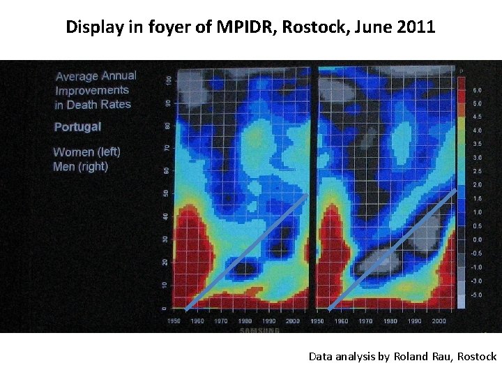
Display in foyer of MPIDR, Rostock, June 2011 Data analysis by Roland Rau, Rostock

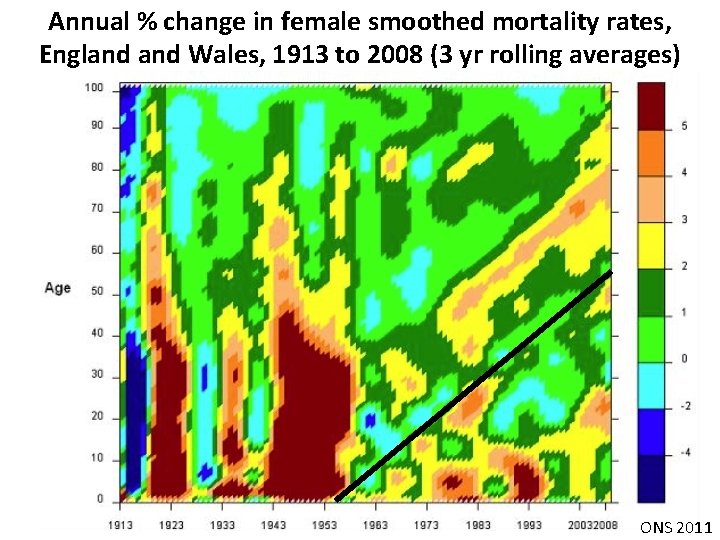
Annual % change in female smoothed mortality rates, England Wales, 1913 to 2008 (3 yr rolling averages) ONS 2011

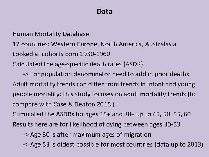
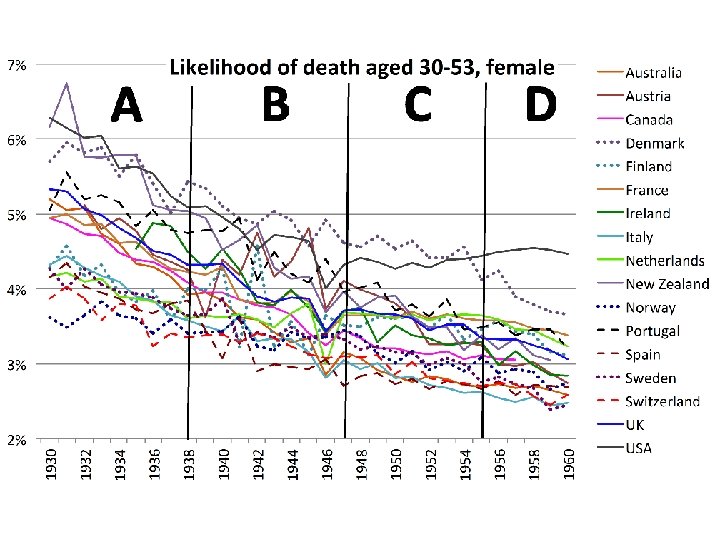
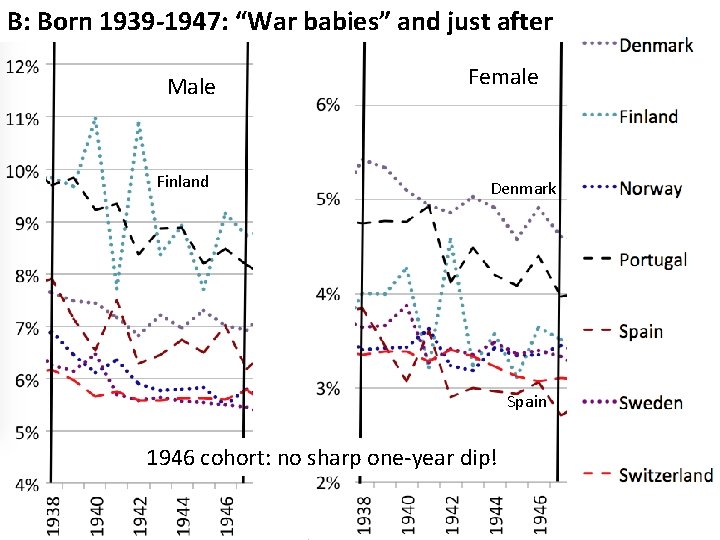
Data Human Mortality Database 17 countries: Western Europe, North America, Australasia Looked at cohorts born 1930 -1960 Calculated the age-specific death rates (ASDR) -> For population denominator need to add in prior deaths Adult mortality trends can differ from trends in infant and young people mortality: this study focuses on adult mortality trends (to compare with Case & Deaton 2015 ) Cumulated the ASDRs for ages 15+ and 30+ up to 45, 50, 55, 60 Results here are for likelihood of dying between ages 30 -53 -> Age 30 is after maximum ages of migration -> Age 53 is oldest possible for most countries (data up to 2013)

Cohort band A: born 1930 -1938 Finland NZ Male Netherlands -> “Golden cohorts”: improving mortality Female Switz

B: Born 1939 -1947: “War babies” and just after Female Male Austria Italy 1946 cohort: sharp one-year dip

B: Born 1939 -1947: “War babies” and just after Male Finland Female Denmark Spain 1946 cohort: no sharp one-year dip!

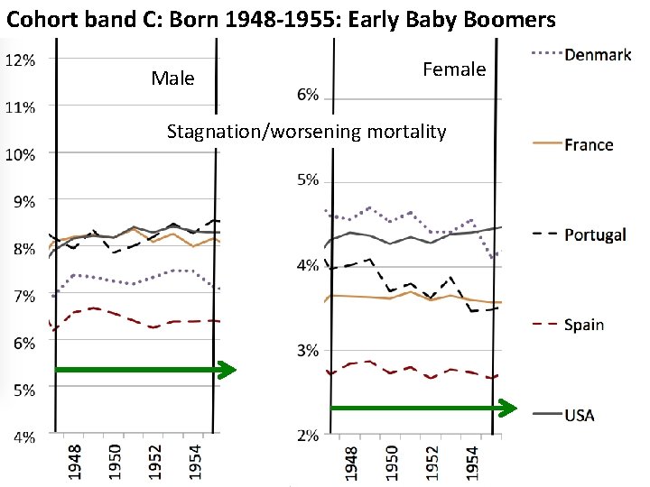
Cohort band C: Born 1948 -1955: Early Baby Boomers Male Female Stagnation/worsening mortality

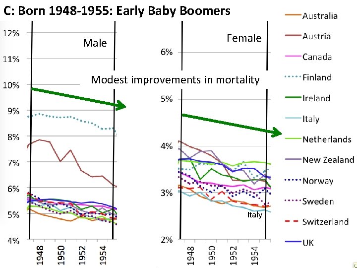
C: Born 1948 -1955: Early Baby Boomers Male Female Modest improvements in mortality Italy

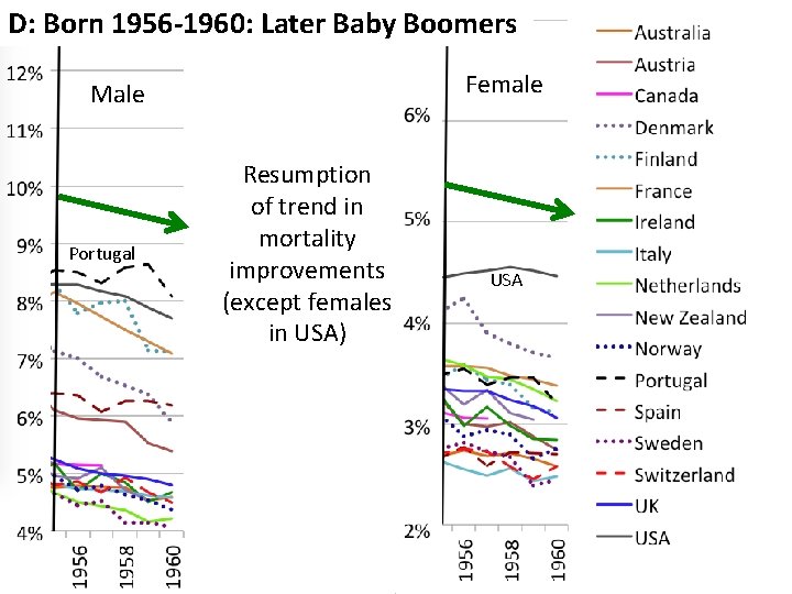
D: Born 1956 -1960: Later Baby Boomers Female Male Portugal Resumption of trend in mortality improvements (except females in USA) USA

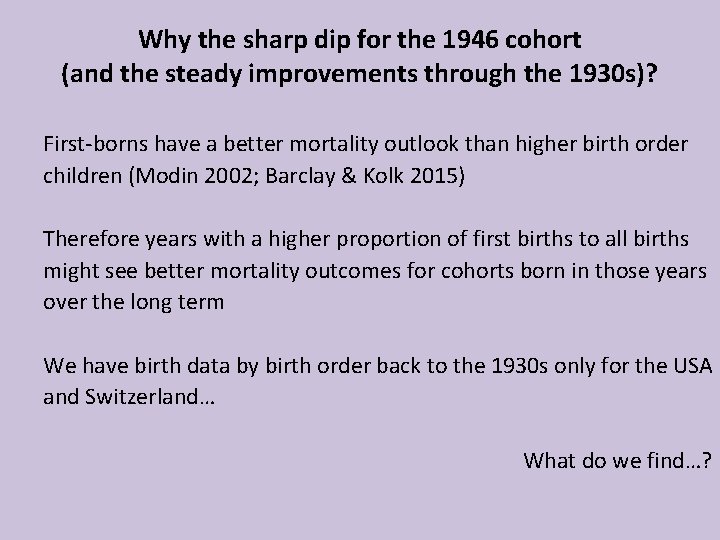
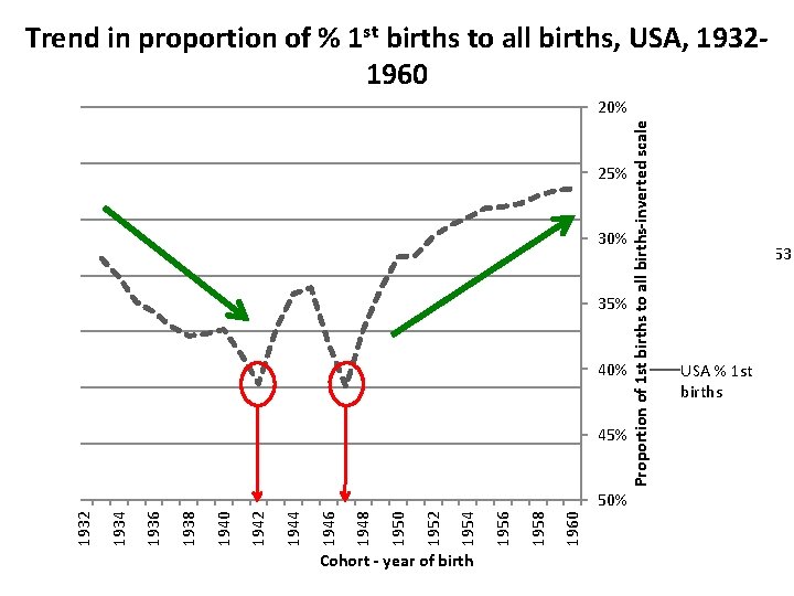
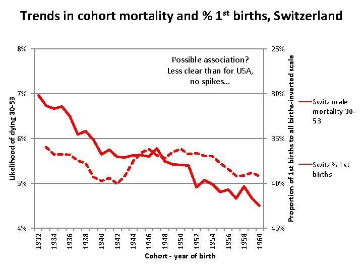
Why the sharp dip for the 1946 cohort (and the steady improvements through the 1930 s)? First-borns have a better mortality outlook than higher birth order children (Modin 2002; Barclay & Kolk 2015) Therefore years with a higher proportion of first births to all births might see better mortality outcomes for cohorts born in those years over the long term We have birth data by birth order back to the 1930 s only for the USA and Switzerland… What do we find…?

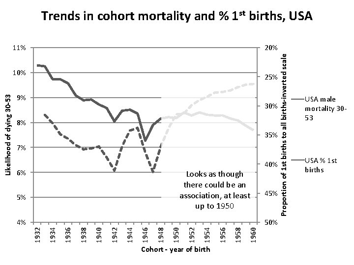
Trends in male mortality, USA, cohorts 1932 -1960 20% 25% 9% 30% 8% 35% 7% 40% 6% 45% 5% Cohort - year of birth 1960 1958 1956 1954 1952 1950 1948 1946 1944 1942 1940 1938 1936 50% 1934 4% 1932 Likelihood of dying 30 -53 10% Proportion of 1 st births to all births-inverted scale 11% USA male mortality 3053 USA % 1 st births

Trend in proportion of % 1 st births to all births, USA, 19321960 20% 25% 9% 30% 8% 35% 7% 40% 6% 45% 5% Cohort - year of birth 1960 1958 1956 1954 1952 1950 1948 1946 1944 1942 1940 1938 1936 50% 1934 4% 1932 Likelihood of dying 30 -53 10% Proportion of 1 st births to all births-inverted scale 11% USA male mortality 30 -53 USA % 1 st births

Trends in cohort mortality and % 1 st births, USA 20% 25% 9% 30% 8% 35% 7% 6% Looks as though there could be an association, at least up to 1950 5% 40% 45% Cohort - year of birth 1960 1958 1956 1954 1952 1950 1948 1946 1944 1942 1940 1938 1936 50% 1934 4% 1932 Likelihood of dying 30 -53 10% Proportion of 1 st births to all births-inverted scale 11% USA male mortality 3053 USA % 1 st births

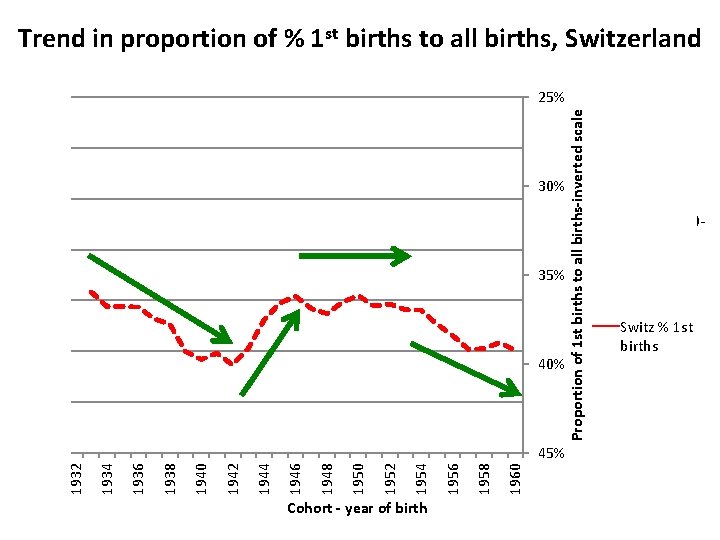
Trend in proportion of % 1 st births to all births, Switzerland 25% 30% 9% 8% 35% 7% 6% 40% 5% Cohort - year of birth 1960 1958 1956 1954 1952 1950 1948 1946 1944 1942 1940 1938 1936 45% 1934 4% 1932 Likelihood of dying 30 -53 10% Proportion of 1 st births to all births-inverted scale 11% Switz male mortality 3053 Switz % 1 st births

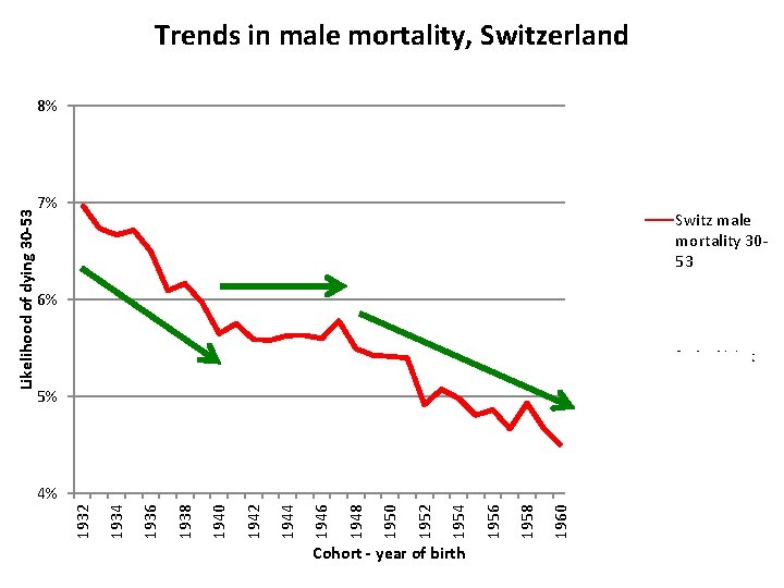
Cohort - year of birth 1960 1958 1956 1954 1952 1950 1948 1946 1944 1942 1940 1938 1936 1934 1932 Likelihood of dying 30 -53 8% 25% 7% 30% 6% 35% 40% 5% 4% 50% Proportion of 1 st births to all births-inverted scale Trends in male mortality, Switzerland 20% Switz male mortality 3053 Switz % 1 st births

Trends in cohort mortality and % 1 st births, Switzerland 25% 7% 30% 6% 35% Cohort - year of birth 1960 1958 1956 1954 1952 1950 1948 1946 1944 1942 1940 45% 1938 4% 1936 40% 1934 5% 1932 Likelihood of dying 30 -53 Possible association? Less clear than for USA, no spikes… Proportion of 1 st births to all births-inverted scale 8% Switz male mortality 3053 Switz % 1 st births

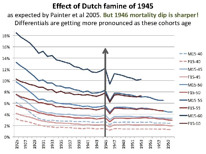
Effect of Dutch famine of 1945 as expected by Painter et al 2005. But 1946 mortality dip is sharper! Differentials are getting more pronounced as these cohorts age

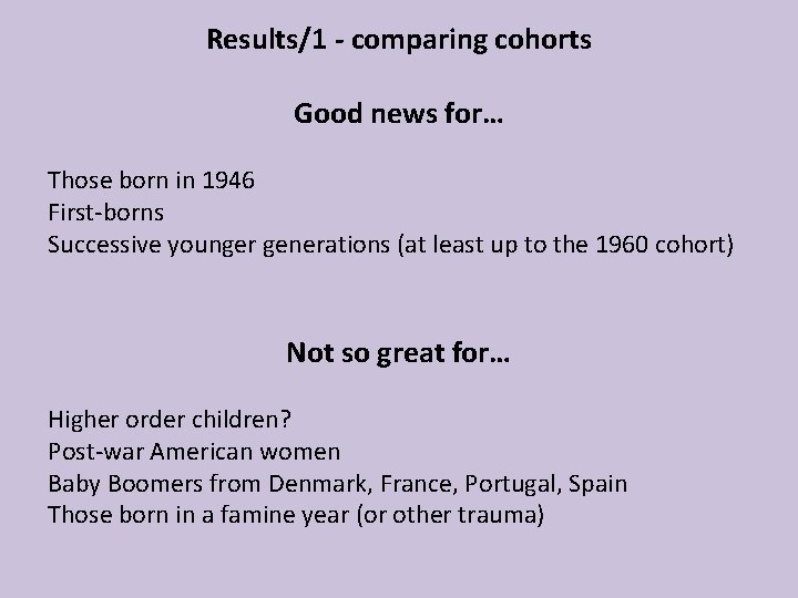
Results/1 - comparing cohorts Good news for… Those born in 1946 First-borns Successive younger generations (at least up to the 1960 cohort) Not so great for… Higher order children? Post-war American women Baby Boomers from Denmark, France, Portugal, Spain Those born in a famine year (or other trauma)

Results/2 A problem with mortality improvement formulae… They compare one year with another one, sometimes 10 years previously. If that year was odd (e. g. 1946) then the mortality improvement would also be odd (->1956 would look bad) Mortality rates often involve smoothing (as rates are so low for younger people). But when the data is smoothed you lose the possibility of seeing spikes or dips for individual years The method I have used (cumulative mortality over a defined age band) is one possible solution to these problems

Thank you! drmarionb@gmail. com