Aerosol Physics and Particle Control PM Particle Shape

Aerosol Physics and Particle Control

PM Particle Shape: -can be found in spherical, rectangular, fiber, or many other irregular shape -shape is important. Affects: -particle behavior -transportation -control technology -effect on the respirotary system (fiber shaped particles particularly harmful to the lungs when they are inhaled, since it is more difficult to remove once they are settled or have clung to air ways.

PM • Muallimköy ortam havasından toplanan partiküllere ait SEM fotorafı

Particle Size • The most important parameters since it affects: – Behavior – Transport – Health effects – Control technology selection Very large range from 0. 01 mm to 100 mm A dust fall following a volcano contains large particles in the range of millimeters that can settle down in a few hours and smal particles (um range) can stay airborne for months.

Human Respiratory System 3 major regions: 1. Head airways region 2. Tracheobronchial region (thoracic) 3. Pulmonary or alveolar region O 2 –CO 2 transfer take place in the pulmonary region. For an adult total area of this gas exchange region is 75 m 2 and total length of the pulmonary vessels is about 2, 000 km. An adult person breathes about 10 -20 times per minute and inhales about 10 -20 liters of air/min.

Particle Size Categories • Based on behavior in the human respiratory system 3 categories can be defined: – Inhalable particles – Thoracic particles – Respirable particles

Particle Size Categories Particles Size Range Total Inhalable (inspirable) All sizes of particles in the air of concern 100 mm ≥ Thoracic 10 mm ≥ Respirable 4 mm ≥ PM 10 10 mm ≥ PM 2. 5 mm ≥

Inhaled Particle Deposition in Human Respiratory System total Head airways Upper bronchial Lower bronchial Alveolar • Deposition of Inhaled Particles in the Human Respiratory Tract and Consequences for Regional Targeting in Respiratory Drug Delivery, Joachim Heyder

Size Distribution • Particle Diameter The highly irregular shape together with the different densities depending on the composition of the particle complicates its size definition. A particle’s size refers to its diameter There are various definitions for the diameter.

Size Distribution • 1. 2. 3. Particle Diameter Equivalent volume diameter Stokes diameter Aerodynamic diameter

Particle Diameter 1. Equivalent volume diameter (de): diameter of a sphere that would have the same volume and density as the particle Assume that following irregular shape has a volume of V, de will be the diameter of sphere whose volume equals to V.

Particle Diameter 2. Stokes diameter (ds): diameter of the sphere that would have the same density and settling velocity as the particle.

Particle Diameter 3. Aerodynamic diameter (da): diameter of the sphere with a standard density (1. 000 kg/m 3) that would have the same settling velocity as the particle

Particle Diameter de only standardizes the shape of the particle by its equivalent spherical volume ds standardizes the settling velocity of the particle but not the density da standardizes both the settling velocity and the particle density. Thus da is a convenient variable to use to analyze particle behavior and design of particle control equipment

Particle Size Distribution

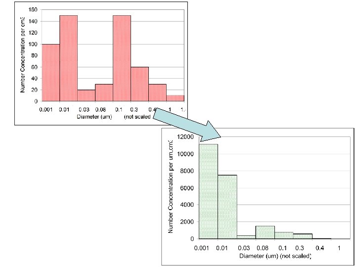
How to display particle size distribution? 0. 02 0. 20

When shown as written in the table, we see that number of particles with diameter between 0. 01 0. 03 um equals to particles with diameter between 0. 1 and 0. 3 um however, diameter range in the first one is only 0. 02 um while in the second is 0. 2 um (1000 times bigger than the first range) 0. 02 0. 20

The area of each rectangular gives the number of particles between Dp 2 and Dp 1 (Ni) Ni = ni ΔDp ni = the value of the number size distribution function (#/μm/cm 3) ΔDp = Dp 2 -Dp 1 (μm)

Let n(Dp) denote the continous function of size distribution n(Dp) d. Dp = Particle concentration with the diameters between Dp and Dp + d. Dp (#/cm 3) n(Dp) (/um/cm 3) • Infinitely small ΔDp d. Dp Dp, um Typical display of distribution function n(Dp)

Normalized Size Distributions • Normalized size distribution ( obtained by: ) can be The fraction of particles with diameters between Dp and Dp + d. Dp to the total number of particles in one cm 3 air Unit of normalized number distribution: μm-1

Surface Area, Volume and Mass Distributions • Surface area distribution ns(Dp) • Mass distribution m(Dp) Y: Characteristic function

Characteristic Functions for Particle Size Distributions (Y(Dp))* Y Y(Dp) Number of particle (Np) 1 Length (Lp) Dp Surface area (Sp) πDp 2 Volume (Vp) 1/6πDp 3 Mass (mp) 1/6πDp 3ρp *assuming particles are spherical

Logaritmic Size Distributions • Since particles’ sizes vary over a very large range, use of logaritmic scale for Dp is more appropriate.

Log Scale Size Distributions Number of particles with diameters between log. Dp and log. Dp + dlog. Dp

Number Surface Volume Seinfeld ve Pandis

Parameters of particle size distributions 1. Mean: Averaged diameter of the sampled particle stream (number distribution) N= Total number of particles (mass distribution) m. T = Total mass of particles

2. Median: taneciklerin %50’sinin büyük, %50’sinin küçük olduğu çap değeri 3. Mode: The most frequent diameter

Beside mean values, it is important to know the how distribution differs from these mean values. For all three distribution shown above, the mean diameters are the same while distribution width is different.

Variance Standard deviation: a measure of the distrubition width Standard Deviation=

Normal (Gaussian) Distribution Normal Distribution Function The mean of the population

Normal (Gaussian) Distribution Standard deviation (s) gives the characteristic width of the symetric number size distribution. 68. 2% of the particles are between dp, mean –s and dp, mean + s, 84. 1% of it with diameters smaller than dpmean+s , and 15. 9% of it with diameters smaller than dpmean-s.

Are the particles in various air streams show a normal distribution?

Log-Normal Dağılım They mostly show a lognormal distribution Dp, g=0. 4μm σg=2. 5 Asıltı parçacıkların %68. 2’si Dpg/σg ile Dpgσg arasındadır. For lognormal distributions, Dpg =Dp, median

Geometrik Ortalama ve Geometrik Standart Sapma

Tanecik Boyut Dağılımının Log. Olasılık Kağıtta Gösterimi taneciklerin %50’sinin küçük olduğu çap Çap, um (Dp, 50) Belirtilen Boyuttan Daha Küçük Olma Yüzdesi

Tanecik Boyut Dağılımının Log. Olasılık Kağıtta Gösterimi Eğer dağılımdan hesaplanan noktalar bir doğru oluşturuyorsa dağılımın lognormal olduğu söylenebilir. Çap, um Tane sayısı, alanı, hacmi veya kütlesi için oluşturulabilir ve her dağılım için %50’sinin küçük olduğu çap bulunabilir. Örnek: Dpg = 0. 5 mm ise, bu taneciklerin %50 sinin bu çaptan küçük olması demektir. 100 tanecik varsa toplam , 50’sinin çapı 0. 5 mm’nin altındadır. Belirtilen Boyuttan Daha Küçük Olma Yüzdesi

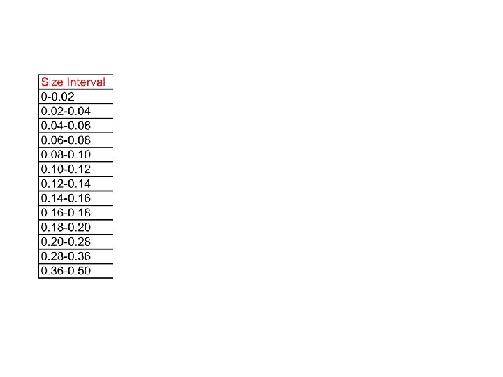
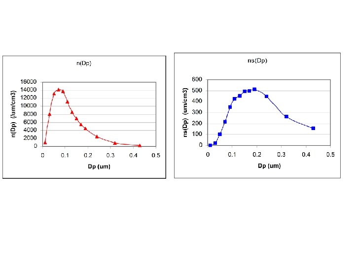
Örnek a) Tane sayısı (n(Dp) ve yüzey alan boyut dağılımını çizin (ns(Dp). Dağılımları karşılaştırın. b) Bu örneklenmiş asılı taneciklerin log-normal bir dağılım gösterdiği söylenebilir mi?

b) Bu dağılım log-normal mi?

σg=Dp, 84. 1/Dp, 50 = 2. 0 0. 16 Dpg=0. 08

Moudi Impactor for Mass Size Distribution

Optical Particle Counter

Differential Mobility Analyzer

Aerodynamic Aerosol Sizer (APS)

Motion of Particles in a Fluid In all particle control technologies, particles are separated from the surrounding fluid by the application of one ore more forces: -gravitational -inertial -centrifugal -electrostatic Those forces cause the accelarate the particles away from the direction of the mean fluid flow, toward the direction of the net force The particles must then be collected and removed from the system to prevent ultimate re-entrainment into the fluid Therefore we need to know the dynamics of particles in fluids

Motion of Particles in a Fluid

Drag Force • FD = CDApp. Fv 2 r – FD=Drag force, N – CD=Drag coefficient – Ap=Projected area of particle, m 2 – p. F=Density of fluid, kg/m 3 – vr= relative velocity, m/s Drag coefficient must be determined experimentally since CD = f(particle shape and the flow regime characterized by Reynolds number)

Stokes’ Law

Motion of Particles in a Fluid

Motion of Particles in a Fluid

Motion of Particles in a Fluid

Motion of Particles in a Fluid

Motion of Particles in a Fluid Note: Continous Fluid A continuum is a region of spacee where charactheristic flow scales L are large enough that properties like density and velocity can be assumed to vary smoothly and therefore have point values. Characteristic scale in diffusion or sedimentation for an aerosol particle is its diameter d A continuum can be assumed if N: number of molecules per unit volume. In water N is about 3. 3 x 1028/m 3, in air N is 2. 5 x 1025 /m 3. It is almost safe to assume a continuum in liquids but not in gases.

Motion of Particles in a Fluid Note: Continous Fluid So does the aerosol particle sense a continuum or a series of discrete bombardements by the air molecules? This can be judged by calculating Knudsen number. d When the Knudsen number is much less than unity (Kn<<1) a continuum can be assumed.

Motion of Particles in a Fluid

Motion of Particles in a Fluid dp>0. 1 um C=1+2. 52 l/dp

Motion of Particles in a Fluid If STP condition is not valid the value of l would change. STP: STP is 0 °C (32 °F or 273 Kelvin) and 1 atm (101. 335 k. Pa, 14. 7 PSI, 760 mm. Hg) Example: At the top of a mountain, the atmospheric pressure is measured as 70 k. Pa, and T as -20 C. What would the error of the slip correction factor be for a 0. 3 um particle if the effect of P and T on l is ignored? Solution: Without considering the effect of T and P C=1 + 2. 52 l/dp = 1. 55 When the effect of Pa nd T is taken into account: l= P 0 T/PT 0 l 0 =1. 34 l 0

Motion of Particles in a Fluid Re>0. 1

Motion of Particles in a Fluid

Motion of Particles in a Fluid

Motion of Particles in a Fluid

Example • A grain of concrete dust particle is falling down onto the floor through room air. The particle diameter is 2 um and the particle density is 2500 kg/m 3. Assuming the room air is still, determine the terminal settling velocity of the particles. The room air is at standard conditions.

Solution • First calculate the slip correction factor for the 2 um particle. • At STP air viscosity=1. 81 x 10 -5 (Ns/m 2), air mean free path l=0. 066 um and air density p=1. 2 kg/m 3 • C = 1 + 2. 52 l/dp=1. 08 • vt = ppdp 2 g. C/18 m=0. 00026 m/s=0. 26 mm/s

Nonspherical Particles and Dynamic Shape Factor • Most particle in practice are nonspherical. Particle dynamic shape factor is defined as the ratio of the actual resistance force of a nonspherical particle to the resistance force of a spherical particle that has the same equivalent volume diameter (de) and the same settling velocity as the nonspherical particle. • Shape factor = FD/3 pmvt. Cde • Where FD is the actual drag force exerted on the nonspherical particle and C is the slp correction factor for de. The dynamic shape factor is always greater than 1 except for certain streamlined shapes.

Shape Dynamic Shape Factor, x Sphere 1. 00 Cube 1. 08 Nonspherical Fiber Clustered Spheres Particles and 2 chain Dynamic Shape 3 chain 5 chain Factor 10 chain 3 compact 1. 06 1. 12 1. 27 1. 35 1. 68 1. 15 Dust Bituminous coal 1. 08 Quartz 1. 36 Sand 1. 57

Aerodynamic Diameter • In reality it is extremely difficult to measure or calculate the equivalent volume diameters and shape factors. • Thus we need an equivalent diameter that can be physically determined and can be used to characterize the particle behavior • Aerodynamic diameter, da, is defined as the diameter of a sphere with unit density (1000 kg/m 3) and the same settling velocity as the particle concern.

Aerodynamic Diameter • Where Cca and Cce are slip correction factors for da and de, respectively. p 0=1000 kg/m 3 • For nonspherical particles, da then: • For spherical particles:

Aerodynamic Diameter • • An irregular particle de =10 mm rp = 3000 kg/m 3 c =1. 3 vt: =0. 0084 m/s • The aerodynamic equivalent sphere • da=15. 2 mm • rp=1000 kg/m 3 vt: =0. 0084 m/s

Aerodynamic Diameter • Particles with dp > 3 mm, the slip effect is negligible so: for nonspherical particles, (de>3 mm) for spherical particles, (dp>3 mm)

Aerodynamic Diameter • For particles with diameter smaller than 3 mm, slip effect must be considered. For non-spherical particles and 0. 1 mm<de<3 mm Aerodynamic diameterfor particles with diameter smaller than 0. 1 mm can be solved using iteration methods. In general those particles behave like gases for which diffusion transport becomes more important than aerodynamic behavior.

Nonsteady State Particle Motion settling velocity

Nonsteady State Particle Motion

Nonsteady State Particle Motion

Nonsteady State Particle Motion

Nonsteady State Particle Motion

Nonsteady State Particle Motion Stopping distance of a particle in a gas flow: a simple means of explaining impaction, answers how important a particle’s inertia is, relative to the viscous effects of the fluid through which it moves Collection of particles (when a flowing fluid approaches a stationary object such as a fabric filter thread, a large water droplet, or a metal plate the fluid flow streamlines will diverge around that object) on a stationary object occur with three different mechanisms Impaction, interception, and diffusion:

Nonsteady State Particle Motion Now assume a sphere in the Stokes regime is projected with an initial velocity of V 0 into a motionless fluid and ignore all but drag force: Take equaiton 3 but assume no gravitational and buoyoncy force:

Nonsteady State Particle Motion

Nonsteady State Particle Motion Above equation is valid only for Stokes region. When Rep>1, the stopping distance is shorter than is predicted by this equation since drag force increases as the Rep increases. This increase in drag force attenuates the velocity of the particle, and hence reduces the stopping distance. Since the Rep is proportional to the particle velocity and the drag force is proportional to the V 2, it is extremely difficult to obtain stopping distance outside of Stokes region. Mercer (1973), proposed an emprical equation to calculate S within %3 accuracy. (for 1<Rep 0<1500)

Nonsteady State Particle Motion If r’ is small, S (xstop) is also small. For instance if a 1 um particle with unit density is projected at 10 m/s into air, it will stop after traveling 36 um An impaction parameter NI can be defined as the ratio of the stopping distance of a particle (based on upstream fluid velocity) to the diameter of the stationary object, or NI=xstop/d 0 If NI is large most of the particles wil impact the ojbect. If NI is very small most of the particles will follow the fluid flow around the object.

Nonsteady State Particle Motion

Example 2 • Calculate the stopping distance of a particle with an aerodynamic diameter of 20 mm in still air. Assume the initial velcoity of the particles is 5 m/s. What would the error be if the particle motion were assumed to be in Stokes region?

Solution • The initial particle Reynolds number: Since Re>1, S = 0. 0046 m

Solution • If the particle were assumed to be in Stokes region, then S The error then would be 0. 00614 -0. 0046/0. 0046=33%