Advanced Valuation Aswath Damodaran www damodaran com Aswath

Advanced Valuation Aswath Damodaran www. damodaran. com Aswath Damodaran 1

Some Initial Thoughts " One hundred thousand lemmings cannot be wrong" Graffiti Aswath Damodaran 2

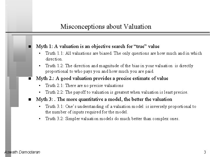
Misconceptions about Valuation Myth 1: A valuation is an objective search for “true” value • • Myth 2. : A good valuation provides a precise estimate of value • • Truth 1. 1: All valuations are biased. The only questions are how much and in which direction. Truth 1. 2: The direction and magnitude of the bias in your valuation is directly proportional to who pays you and how much you are paid. Truth 2. 1: There are no precise valuations Truth 2. 2: The payoff to valuation is greatest when valuation is least precise. Myth 3: . The more quantitative a model, the better the valuation • • Aswath Damodaran Truth 3. 1: One’s understanding of a valuation model is inversely proportional to the number of inputs required for the model. Truth 3. 2: Simpler valuation models do much better than complex ones. 3

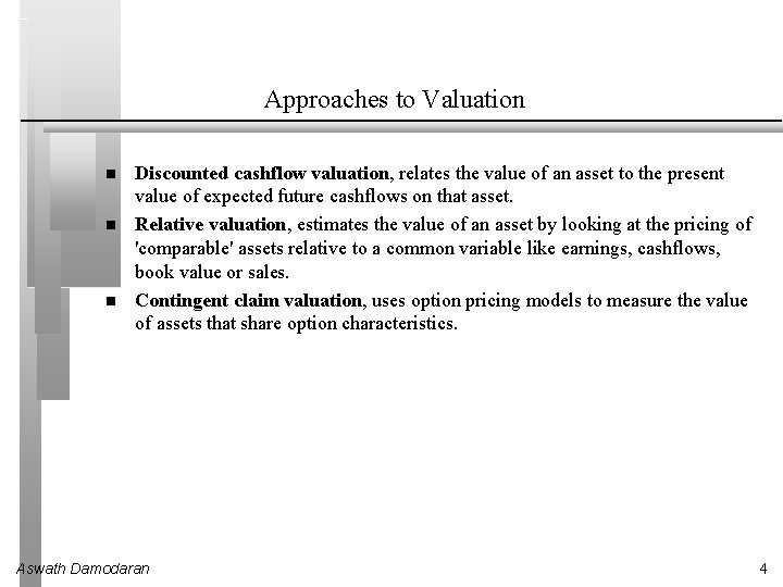
Approaches to Valuation Discounted cashflow valuation, relates the value of an asset to the present value of expected future cashflows on that asset. Relative valuation, estimates the value of an asset by looking at the pricing of 'comparable' assets relative to a common variable like earnings, cashflows, book value or sales. Contingent claim valuation, uses option pricing models to measure the value of assets that share option characteristics. Aswath Damodaran 4

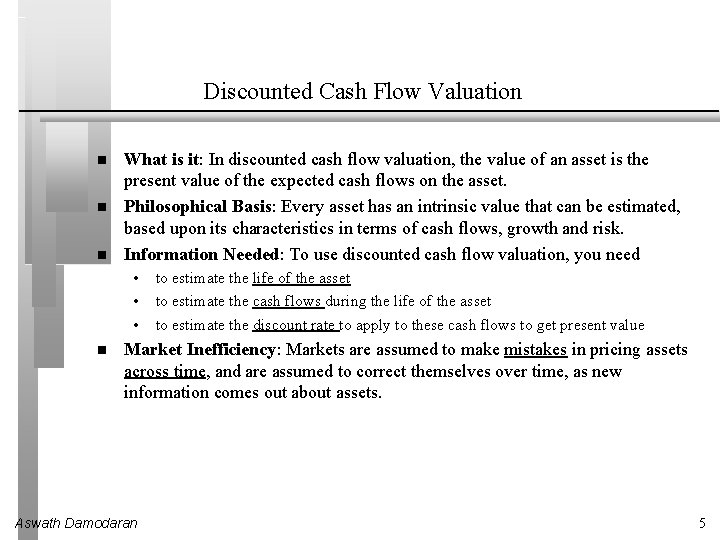
Discounted Cash Flow Valuation What is it: In discounted cash flow valuation, the value of an asset is the present value of the expected cash flows on the asset. Philosophical Basis: Every asset has an intrinsic value that can be estimated, based upon its characteristics in terms of cash flows, growth and risk. Information Needed: To use discounted cash flow valuation, you need • • • to estimate the life of the asset to estimate the cash flows during the life of the asset to estimate the discount rate to apply to these cash flows to get present value Market Inefficiency: Markets are assumed to make mistakes in pricing assets across time, and are assumed to correct themselves over time, as new information comes out about assets. Aswath Damodaran 5

DCF Choices: Equity Valuation versus Firm Valuation: Value the entire business Equity valuation: Value just the equity claim in the business Aswath Damodaran 6

The Drivers of Value… Aswath Damodaran 7

Aswath Damodaran 8

Aswath Damodaran 9

Aswath Damodaran 10

Aswath Damodaran 11

Aswath Damodaran 12

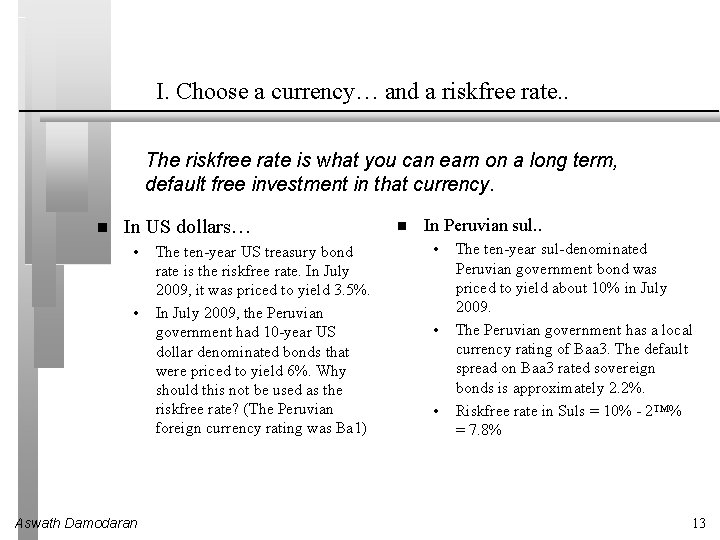
I. Choose a currency… and a riskfree rate. . The riskfree rate is what you can earn on a long term, default free investment in that currency. In US dollars… • • Aswath Damodaran The ten-year US treasury bond rate is the riskfree rate. In July 2009, it was priced to yield 3. 5%. In July 2009, the Peruvian government had 10 -year US dollar denominated bonds that were priced to yield 6%. Why should this not be used as the riskfree rate? (The Peruvian foreign currency rating was Ba 1) In Peruvian sul. . • • • The ten-year sul-denominated Peruvian government bond was priced to yield about 10% in July 2009. The Peruvian government has a local currency rating of Baa 3. The default spread on Baa 3 rated sovereign bonds is approximately 2. 2%. Riskfree rate in Suls = 10% - 2™% = 7. 8% 13

Aswath Damodaran 14

II. Measure earnings right. . Aswath Damodaran 15

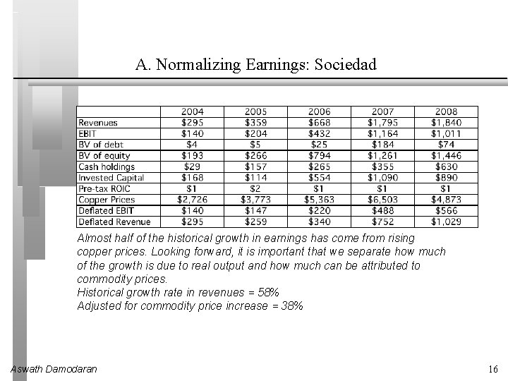
A. Normalizing Earnings: Sociedad Almost half of the historical growth in earnings has come from rising copper prices. Looking forward, it is important that we separate how much of the growth is due to real output and how much can be attributed to commodity prices. Historical growth rate in revenues = 58% Adjusted for commodity price increase = 38% Aswath Damodaran 16

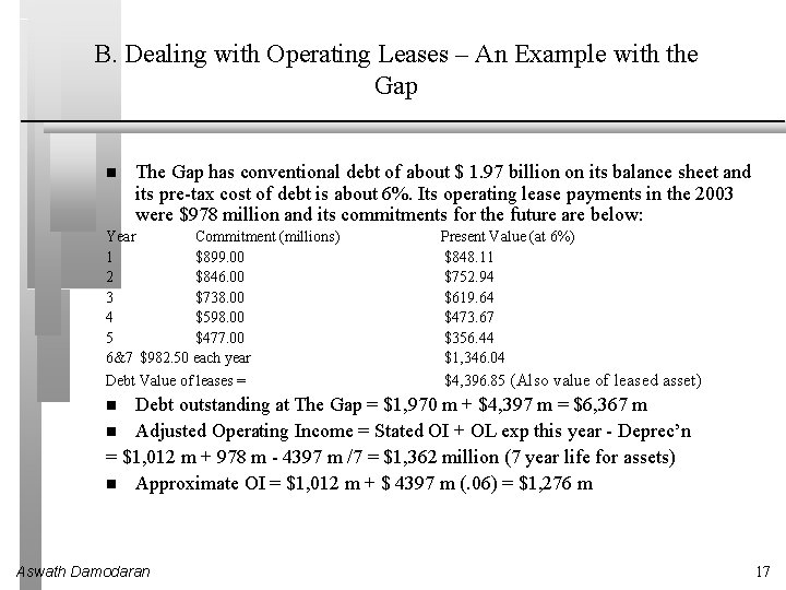
B. Dealing with Operating Leases – An Example with the Gap The Gap has conventional debt of about $ 1. 97 billion on its balance sheet and its pre-tax cost of debt is about 6%. Its operating lease payments in the 2003 were $978 million and its commitments for the future are below: Year Commitment (millions) 1 $899. 00 2 $846. 00 3 $738. 00 4 $598. 00 5 $477. 00 6&7 $982. 50 each year Debt Value of leases = Present Value (at 6%) $848. 11 $752. 94 $619. 64 $473. 67 $356. 44 $1, 346. 04 $4, 396. 85 (Also value of leased asset) Debt outstanding at The Gap = $1, 970 m + $4, 397 m = $6, 367 m Adjusted Operating Income = Stated OI + OL exp this year - Deprec’n = $1, 012 m + 978 m - 4397 m /7 = $1, 362 million (7 year life for assets) Approximate OI = $1, 012 m + $ 4397 m (. 06) = $1, 276 m Aswath Damodaran 17

The Collateral Effects of Treating Operating Leases as Debt Aswath Damodaran 18

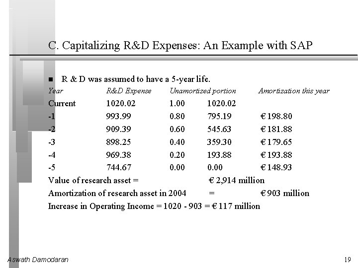
C. Capitalizing R&D Expenses: An Example with SAP R & D was assumed to have a 5 -year life. Year R&D Expense Unamortized portion Amortization this year Current 1020. 02 1. 00 1020. 02 -1 993. 99 0. 80 795. 19 € 198. 80 -2 909. 39 0. 60 545. 63 € 181. 88 -3 898. 25 0. 40 359. 30 € 179. 65 -4 969. 38 0. 20 193. 88 € 193. 88 -5 744. 67 0. 00 € 148. 93 Value of research asset = € 2, 914 million Amortization of research asset in 2004 = € 903 million Increase in Operating Income = 1020 - 903 = € 117 million Aswath Damodaran 19

The Effect of Capitalizing R&D at SAP Aswath Damodaran 20

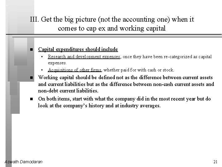
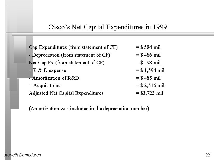
III. Get the big picture (not the accounting one) when it comes to cap ex and working capital Capital expenditures should include • • Research and development expenses, once they have been re-categorized as capital expenses. Acquisitions of other firms, whether paid for with cash or stock. Working capital should be defined not as the difference between current assets and current liabilities but as the difference between non-cash current assets and non-debt current liabilities. On both items, start with what the company did in the most recent year but do look at the company’s history and at industry averages. Aswath Damodaran 21

Cisco’s Net Capital Expenditures in 1999 Cap Expenditures (from statement of CF) - Depreciation (from statement of CF) Net Cap Ex (from statement of CF) + R & D expense - Amortization of R&D + Acquisitions Adjusted Net Capital Expenditures = $ 584 mil = $ 486 mil = $ 98 mil = $ 1, 594 mil = $ 485 mil = $ 2, 516 mil = $3, 723 mil (Amortization was included in the depreciation number) Aswath Damodaran 22

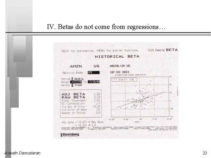
IV. Betas do not come from regressions… Aswath Damodaran 23

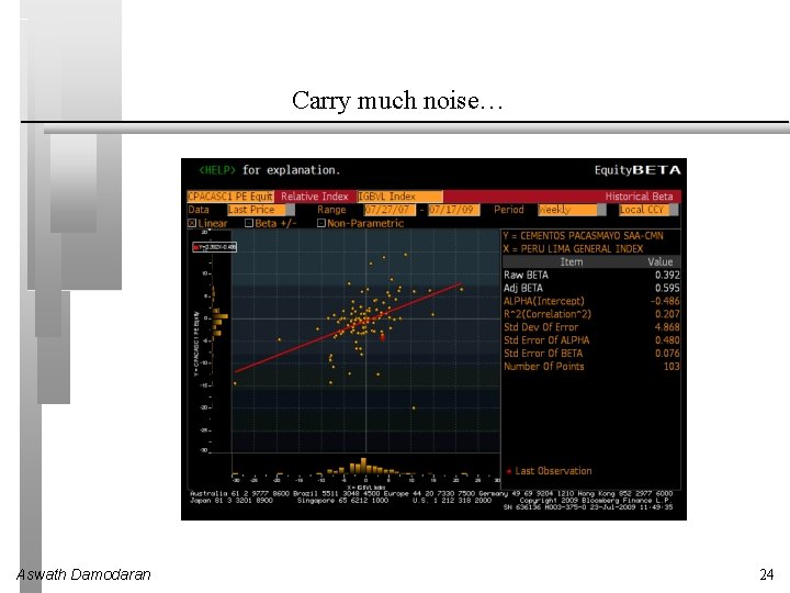
Carry much noise… Aswath Damodaran 24

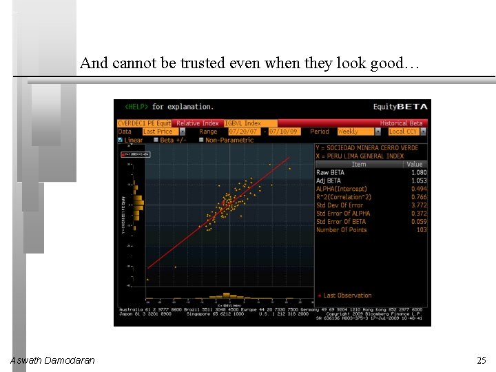
And cannot be trusted even when they look good… Aswath Damodaran 25

Bottom-up Betas Aswath Damodaran 26

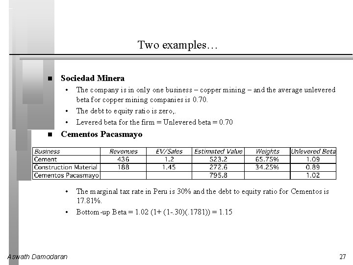
Two examples… Sociedad Minera • • • The company is in only one business – copper mining – and the average unlevered beta for copper mining companies is 0. 70. The debt to equity ratio is zero, . Levered beta for the firm = Unlevered beta = 0. 70 Cementos Pacasmayo • • Aswath Damodaran The marginal tax rate in Peru is 30% and the debt to equity ratio for Cementos is 17. 81%. Bottom-up Beta = 1. 02 (1+ (1 -. 30)(. 1781)) = 1. 15 27

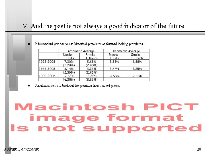
V. And the past is not always a good indicator of the future It is standard practice to use historical premiums as forward looking premiums. : An alternative is to back out the premium from market prices: Aswath Damodaran 28

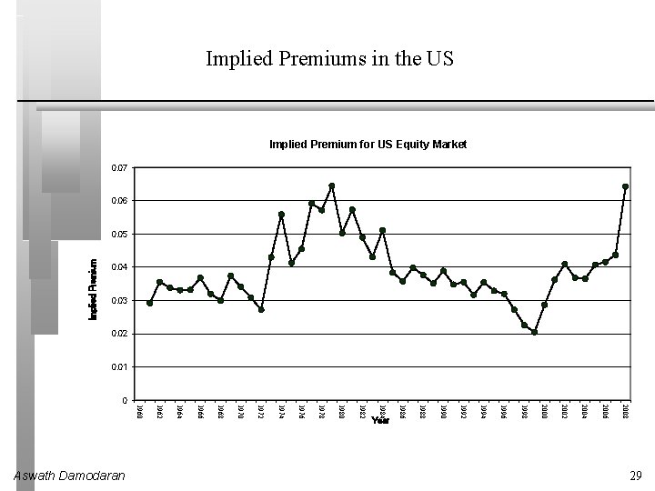
Implied Premiums in the US Implied Premium for US Equity Market 0. 07 0. 06 Implied Premium 0. 05 0. 04 0. 03 0. 02 0. 01 2008 2006 2004 2002 2000 1998 1996 1994 1992 1990 1988 Year 1986 1984 1982 1980 1978 1976 1974 1972 1970 1968 1966 1964 1962 Aswath Damodaran 1960 0 29

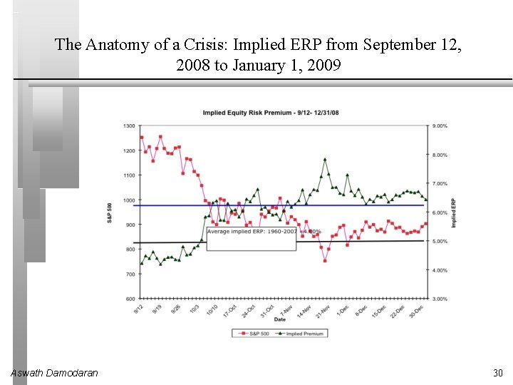
The Anatomy of a Crisis: Implied ERP from September 12, 2008 to January 1, 2009 Aswath Damodaran 30

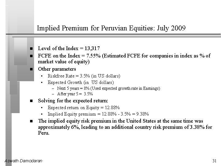
Implied Premium for Peruvian Equities: July 2009 Level of the Index = 13, 317 FCFE on the Index = 7. 55% (Estimated FCFE for companies in index as % of market value of equity) Other parameters • • Riskfree Rate = 3. 5% (in US dollars) Expected Growth (in US dollars) – Next 5 years = 8% (Used expected growth rate in Earnings) – After year 5 = 3. 5% Solving for the expected return: • • Expected return on Equity = 12. 88% Implied Equity premium = 12. 88% - 3. 5% = 9. 38% The implied equity risk premium in the United States at the same time was approximately 6%, leading to an additional country risk premium of 3. 38% for Peru. Aswath Damodaran 31

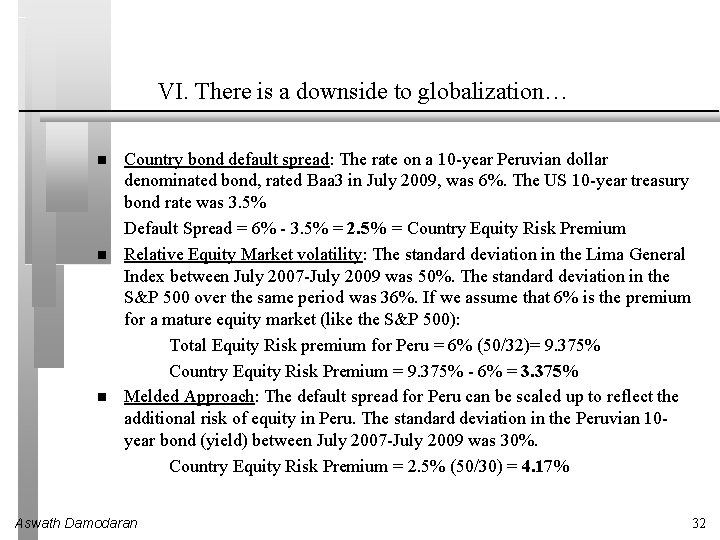
VI. There is a downside to globalization… Country bond default spread: The rate on a 10 -year Peruvian dollar denominated bond, rated Baa 3 in July 2009, was 6%. The US 10 -year treasury bond rate was 3. 5% Default Spread = 6% - 3. 5% = 2. 5% = Country Equity Risk Premium Relative Equity Market volatility: The standard deviation in the Lima General Index between July 2007 -July 2009 was 50%. The standard deviation in the S&P 500 over the same period was 36%. If we assume that 6% is the premium for a mature equity market (like the S&P 500): Total Equity Risk premium for Peru = 6% (50/32)= 9. 375% Country Equity Risk Premium = 9. 375% - 6% = 3. 375% Melded Approach: The default spread for Peru can be scaled up to reflect the additional risk of equity in Peru. The standard deviation in the Peruvian 10 year bond (yield) between July 2007 -July 2009 was 30%. Country Equity Risk Premium = 2. 5% (50/30) = 4. 17% Aswath Damodaran 32

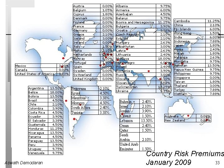
Mexico Canada United States of America Argentina Belize Bolivia Brazil Chile Colombia Costa Rica Ecuador El Salvador Guatemala Honduras Nicaragua Panama Paraguay Peru Uruguay Venezuela Aswath Damodaran 3. 00% 0. 00% 13. 50% 18. 00% 13. 50% 4. 50% 2. 10% 3. 90% 4. 50% 3. 90% 3. 38% 4. 50% 11. 25% 13. 50% 4. 50% 13. 50% 3. 90% 9. 75% Austria Belgium Cyprus Denmark Finland France Germany Greece Iceland Ireland Italy Malta Netherlands Norway Portugal Spain Sweden Switzerland United Kingdom Botswana Egypt Mauritius Morocco South Africa Tunisia 0. 00% 1. 05% 1. 80% 0. 00% 2. 10% 3. 00% 0. 00% 1. 50% 2. 10% 0. 00% 1. 50% 0. 00% 2. 10% 4. 50% 3. 38% 4. 50% 2. 40% 3. 38% Albania Armenia Azerbaijan Belarus Bosnia and Herzegovina Bulgaria Croatia Czech Republic Estonia Hungary Kazakhstan Latvia Lithuania Moldova Montenegro Poland Romania Russia Slovakia Slovenia [1] Turkmenistan Ukraine Bahrain Israel Jordan Kuwait Lebanon Oman Qatar Saudi Arabia United Arab Emirates 2. 40% 2. 10% 3. 90% 1. 50% 13. 50% 2. 40% 1. 50% 9. 75% 6. 00% 4. 50% 9. 75% 11. 25% 3. 90% 3. 38% 2. 10% 2. 63% 3. 00% 2. 63% 2. 40% 18. 00% 6. 00% 2. 40% 3. 90% 3. 00% 2. 10% 1. 50% 11. 25% 9. 75% Cambodia China Fiji Islands Hong Kong India Indonesia Japan Korea Macao Malaysia Mongolia Pakistan Papua New Guinea Philippines Singapore Taiwan Thailand Turkey Vietnam Australia New Zealand 11. 25% 2. 10% 6. 00% 1. 50% 6. 00% 7. 88% 1. 80% 2. 40% 1. 80% 2. 63% 9. 75% 13. 50% 9. 75% 0. 00% 1. 80% 3. 00% 7. 88% 0. 00% 2. 10% 1. 50% Country Risk Premiums 33 January 2009

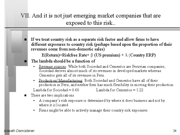
VII. And it is not just emerging market companies that are exposed to this risk. . If we treat country risk as a separate risk factor and allow firms to have different exposures to country risk (perhaps based upon the proportion of their revenues come from non-domestic sales) E(Return)=Riskfree Rate+ b (US premium) + l (Country ERP) The lambda should be a function of • Revenue sources: While both Sociedad and Cementos are Peruvian companies, Sociedad derives almost much of its revenues in developed markets whereas Cementos gets all of its revenues in Peru. • Production/ Manufacturing: Both Sociedad and Cementos have all of their production in Peru, and neither firm has much flexibility in moving their production. Lambda for Sociedad = 0. 60 Lambda for Cementos = 1. 22 There are two implications • A company’s risk exposure is determined by where it does business and not by where it is located • Firms might be able to actively manage their country risk exposures Aswath Damodaran 34

VIII. Growth has to be earned (not endowed or estimated) Aswath Damodaran 35

IX. All good things come to an end. . And the terminal value is not an ATM… Aswath Damodaran 36

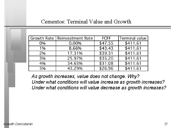
Cementos: Terminal Value and Growth As growth increases, value does not change. Why? Under what conditions will value increase as growth increases? Under what conditions will value decrease as growth increases? Aswath Damodaran 37

X. The loose ends matter… Aswath Damodaran 38

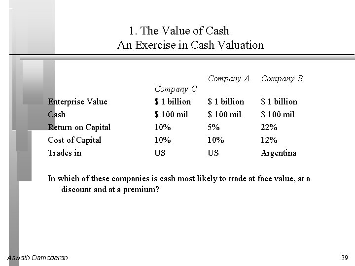
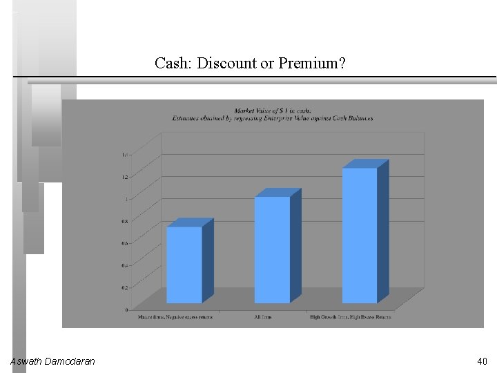
1. The Value of Cash An Exercise in Cash Valuation Enterprise Value Cash Return on Capital Cost of Capital Trades in Company C $ 1 billion $ 100 mil 10% US Company A Company B $ 1 billion $ 100 mil 5% 10% US $ 1 billion $ 100 mil 22% 12% Argentina In which of these companies is cash most likely to trade at face value, at a discount and at a premium? Aswath Damodaran 39

Cash: Discount or Premium? Aswath Damodaran 40

2. Dealing with Holdings in Other firms Holdings in other firms can be categorized into • • • Minority passive holdings, in which case only the dividend from the holdings is shown in the balance sheet Minority active holdings, in which case the share of equity income is shown in the income statements Majority active holdings, in which case the financial statements are consolidated. We tend to be sloppy in practice in dealing with cross holdings. After valuing the operating assets of a firm, using consolidated statements, it is common to add on the balance sheet value of minority holdings (which are in book value terms) and subtract out the minority interests (again in book value terms), representing the portion of the consolidated company that does not belong to the parent company. Aswath Damodaran 41

How to value holdings in other firms. . In a perfect world, we would strip the parent company from its subsidiaries and value each one separately. The value of the combined firm will be • Value of parent company + Proportion of value of each subsidiary To do this right, you will need to be provided detailed information on each subsidiary to estimated cash flows and discount rates. Aswath Damodaran 42

Two compromise solutions… The market value solution: When the subsidiaries are publicly traded, you could use their traded market capitalizations to estimate the values of the cross holdings. You do risk carrying into your valuation any mistakes that the market may be making in valuation. The relative value solution: When there are too many cross holdings to value separately or when there is insufficient information provided on cross holdings, you can convert the book values of holdings that you have on the balance sheet (for both minority holdings and minority interests in majority holdings) by using the average price to book value ratio of the sector in which the subsidiaries operate. Aswath Damodaran 43

3. Other Assets that have not been counted yet. . Unutilized assets: If you have assets or property that are not being utilized (vacant land, for example), you have not valued it yet. You can assess a market value for these assets and add them on to the value of the firm. Overfunded pension plans: If you have a defined benefit plan and your assets exceed your expected liabilities, you could consider the over funding with two caveats: • • Collective bargaining agreements may prevent you from laying claim to these excess assets. There are tax consequences. Often, withdrawals from pension plans get taxed at much higher rates. Do not double count an asset. If you count the income from an asset in your cashflows, you cannot count the market value of the asset in your value. Aswath Damodaran 44

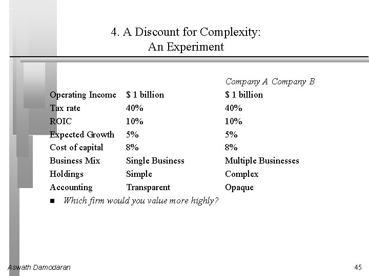
4. A Discount for Complexity: An Experiment Operating Income $ 1 billion Tax rate 40% ROIC 10% Expected Growth 5% Cost of capital 8% Business Mix Single Business Holdings Simple Accounting Transparent Which firm would you value more highly? Aswath Damodaran Company A Company B $ 1 billion 40% 10% 5% 8% Multiple Businesses Complex Opaque 45

Measuring Complexity: Volume of Data in Financial Statements Aswath Damodaran 46

Measuring Complexity: A Complexity Score Aswath Damodaran 47

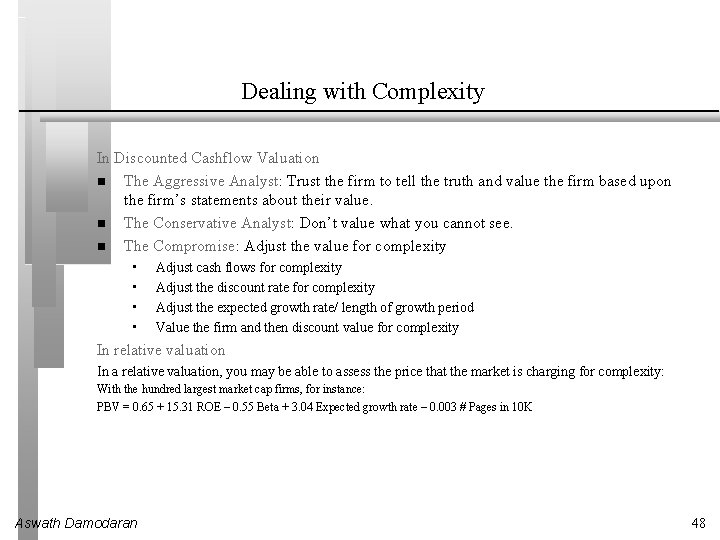
Dealing with Complexity In Discounted Cashflow Valuation The Aggressive Analyst: Trust the firm to tell the truth and value the firm based upon the firm’s statements about their value. The Conservative Analyst: Don’t value what you cannot see. The Compromise: Adjust the value for complexity • • Adjust cash flows for complexity Adjust the discount rate for complexity Adjust the expected growth rate/ length of growth period Value the firm and then discount value for complexity In relative valuation In a relative valuation, you may be able to assess the price that the market is charging for complexity: With the hundred largest market cap firms, for instance: PBV = 0. 65 + 15. 31 ROE – 0. 55 Beta + 3. 04 Expected growth rate – 0. 003 # Pages in 10 K Aswath Damodaran 48

5. The Value of Synergy Aswath Damodaran 49

Valuing Synergy (1) the firms involved in the merger are valued independently, by discounting expected cash flows to each firm at the weighted average cost of capital for that firm. (2) the value of the combined firm, with no synergy, is obtained by adding the values obtained for each firm in the first step. (3) The effects of synergy are built into expected growth rates and cashflows, and the combined firm is re-valued with synergy. Value of Synergy = Value of the combined firm, with synergy - Value of the combined firm, without synergy Aswath Damodaran 50

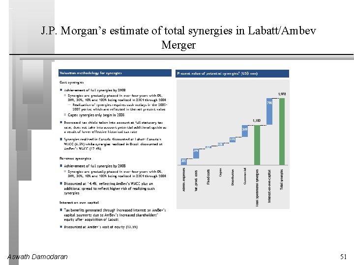
J. P. Morgan’s estimate of total synergies in Labatt/Ambev Merger Aswath Damodaran 51

5. Brand name, great management, superb product …Are we short changing the intangibles? There is often a temptation to add on premiums for intangibles. Among them are • • Brand name Great management Loyal workforce Technological prowess There are two potential dangers: • • For some assets, the value may already be in your value and adding a premium will be double counting. For other assets, the value may be ignored but incorporating it will not be easy. Aswath Damodaran 52

Categorizing Intangibles Aswath Damodaran 53

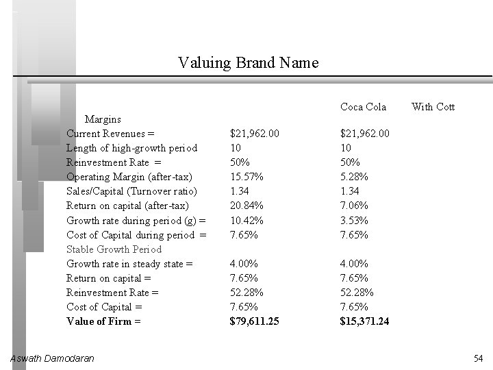
Valuing Brand Name Margins Current Revenues = Length of high-growth period Reinvestment Rate = Operating Margin (after-tax) Sales/Capital (Turnover ratio) Return on capital (after-tax) Growth rate during period (g) = Cost of Capital during period = Stable Growth Period Growth rate in steady state = Return on capital = Reinvestment Rate = Cost of Capital = Value of Firm = Aswath Damodaran Coca Cola $21, 962. 00 10 50% 15. 57% 1. 34 20. 84% 10. 42% 7. 65% $21, 962. 00 10 50% 5. 28% 1. 34 7. 06% 3. 53% 7. 65% 4. 00% 7. 65% 52. 28% 7. 65% $79, 611. 25 4. 00% 7. 65% 52. 28% 7. 65% $15, 371. 24 With Cott 54

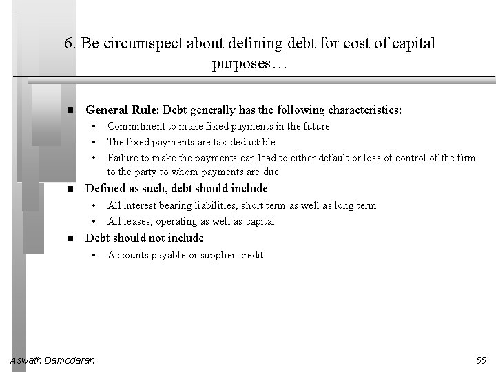
6. Be circumspect about defining debt for cost of capital purposes… General Rule: Debt generally has the following characteristics: • • • Defined as such, debt should include • • Commitment to make fixed payments in the future The fixed payments are tax deductible Failure to make the payments can lead to either default or loss of control of the firm to the party to whom payments are due. All interest bearing liabilities, short term as well as long term All leases, operating as well as capital Debt should not include • Aswath Damodaran Accounts payable or supplier credit 55

But should consider other potential liabilities when getting to equity value… If you have under funded pension fund or health care plans, you should consider the under funding at this stage in getting to the value of equity. • • If you do so, you should not double count by also including a cash flow line item reflecting cash you would need to set aside to meet the unfunded obligation. You should not be counting these items as debt in your cost of capital calculations…. If you have contingent liabilities - for example, a potential liability from a lawsuit that has not been decided - you should consider the expected value of these contingent liabilities • Aswath Damodaran Value of contingent liability = Probability that the liability will occur * Expected value of liability 56

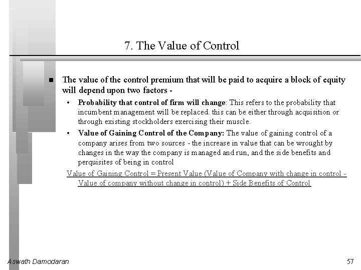
7. The Value of Control The value of the control premium that will be paid to acquire a block of equity will depend upon two factors • Probability that control of firm will change: This refers to the probability that incumbent management will be replaced. this can be either through acquisition or through existing stockholders exercising their muscle. • Value of Gaining Control of the Company: The value of gaining control of a company arises from two sources - the increase in value that can be wrought by changes in the way the company is managed and run, and the side benefits and perquisites of being in control Value of Gaining Control = Present Value (Value of Company with change in control Value of company without change in control) + Side Benefits of Control Aswath Damodaran 57

Aswath Damodaran 58

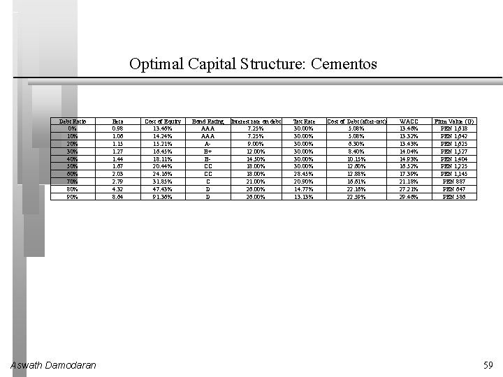
Optimal Capital Structure: Cementos Debt Ratio 0% 10% 20% 30% 40% 50% 60% 70% 80% 90% Aswath Damodaran Beta 0. 98 1. 06 1. 15 1. 27 1. 44 1. 67 2. 03 2. 79 4. 32 8. 64 Cost of Equity 13. 46% 14. 24% 15. 21% 16. 45% 18. 11% 20. 44% 24. 16% 31. 85% 47. 43% 91. 36% Bond Rating AAA AB+ BCC CC C D D Interest rate on debt 7. 25% 9. 00% 12. 00% 14. 50% 18. 00% 21. 00% 26. 00% Tax Rate 30. 00% 28. 45% 20. 90% 14. 77% 13. 13% Cost of Debt (after-tax) 5. 08% 6. 30% 8. 40% 10. 15% 12. 60% 12. 88% 16. 61% 22. 16% 22. 59% WACC 13. 46% 13. 32% 13. 43% 14. 04% 14. 93% 16. 52% 17. 39% 21. 18% 27. 21% 29. 46% Firm Value (G) PEN 1, 618 PEN 1, 642 PEN 1, 625 PEN 1, 527 PEN 1, 404 PEN 1, 225 PEN 1, 145 PEN 887 PEN 647 PEN 586 59

Aswath Damodaran 60

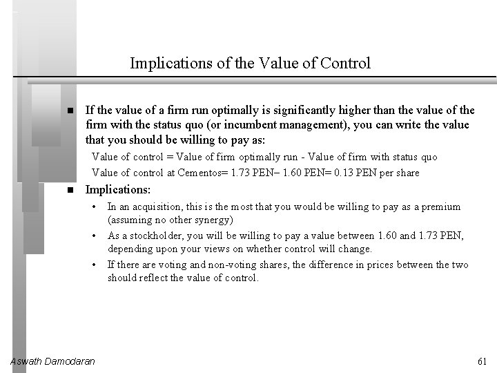
Implications of the Value of Control If the value of a firm run optimally is significantly higher than the value of the firm with the status quo (or incumbent management), you can write the value that you should be willing to pay as: Value of control = Value of firm optimally run - Value of firm with status quo Value of control at Cementos= 1. 73 PEN– 1. 60 PEN= 0. 13 PEN per share Implications: • • • Aswath Damodaran In an acquisition, this is the most that you would be willing to pay as a premium (assuming no other synergy) As a stockholder, you will be willing to pay a value between 1. 60 and 1. 73 PEN, depending upon your views on whether control will change. If there are voting and non-voting shares, the difference in prices between the two should reflect the value of control. 61

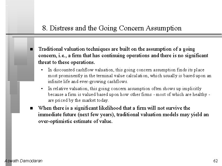
8. Distress and the Going Concern Assumption Traditional valuation techniques are built on the assumption of a going concern, i. e. , a firm that has continuing operations and there is no significant threat to these operations. • • In discounted cashflow valuation, this going concern assumption finds its place most prominently in the terminal value calculation, which usually is based upon an infinite life and ever-growing cashflows. In relative valuation, this going concern assumption often shows up implicitly because a firm is valued based upon how other firms - most of which are healthy are priced by the market today. When there is a significant likelihood that a firm will not survive the immediate future (next few years), traditional valuation models may yield an over-optimistic estimate of value. Aswath Damodaran 62

Aswath Damodaran 63

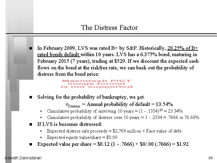
The Distress Factor In February 2009, LVS was rated B+ by S&P. Historically, 28. 25% of B+ rated bonds default within 10 years. LVS has a 6. 375% bond, maturing in February 2015 (7 years), trading at $529. If we discount the expected cash flows on the bond at the riskfree rate, we can back out the probability of distress from the bond price: Solving for the probability of bankruptcy, we get: Distress = Annual probability of default = 13. 54% • • If LVS is becomes distressed: • • Cumulative probability of surviving 10 years = (1 -. 1354)10 = 23. 34% Cumulative probability of distress over 10 years = 1 -. 2334 =. 7666 or 76. 66% Expected distress sale proceeds = $2, 769 million < Face value of debt Expected equity value/share = $0. 00 Expected value per share = $8. 12 (1 -. 7666) + $0/. 00 (. 7666) = $1. 92 Aswath Damodaran 64

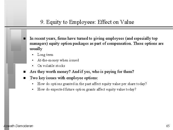
9. Equity to Employees: Effect on Value In recent years, firms have turned to giving employees (and especially top managers) equity option packages as part of compensation. These options are usually • • • Long term At-the-money when issued On volatile stocks Are they worth money? And if yes, who is paying for them? Two key issues with employee options: • • Aswath Damodaran How do options granted in the past affect equity value per share today? How do expected future option grants affect equity value today? 65

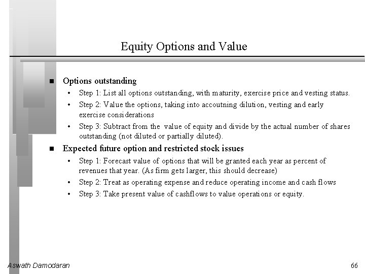
Equity Options and Value Options outstanding • • • Step 1: List all options outstanding, with maturity, exercise price and vesting status. Step 2: Value the options, taking into accoutning dilution, vesting and early exercise considerations Step 3: Subtract from the value of equity and divide by the actual number of shares outstanding (not diluted or partially diluted). Expected future option and restricted stock issues • • • Aswath Damodaran Step 1: Forecast value of options that will be granted each year as percent of revenues that year. (As firm gets larger, this should decrease) Step 2: Treat as operating expense and reduce operating income and cash flows Step 3: Take present value of cashflows to value operations or equity. 66

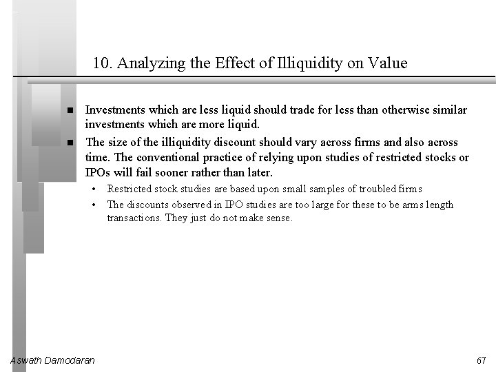
10. Analyzing the Effect of Illiquidity on Value Investments which are less liquid should trade for less than otherwise similar investments which are more liquid. The size of the illiquidity discount should vary across firms and also across time. The conventional practice of relying upon studies of restricted stocks or IPOs will fail sooner rather than later. • • Aswath Damodaran Restricted stock studies are based upon small samples of troubled firms The discounts observed in IPO studies are too large for these to be arms length transactions. They just do not make sense. 67

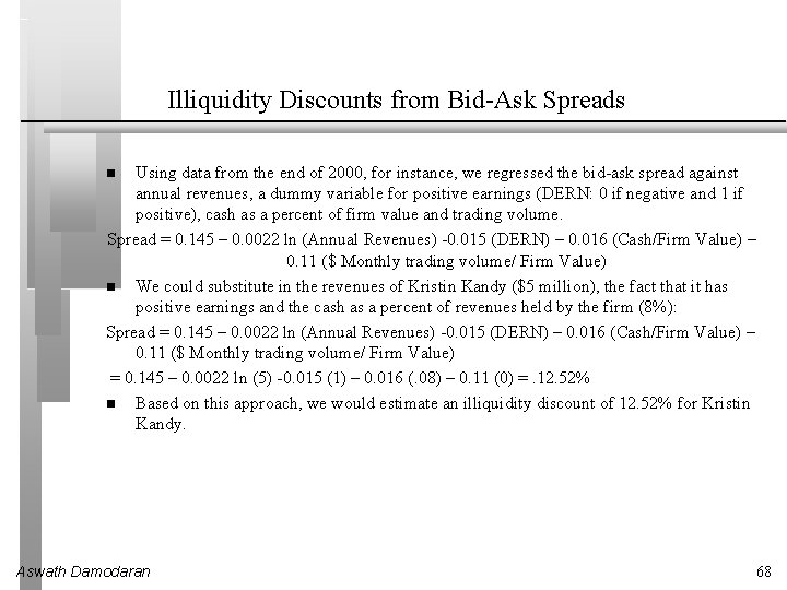
Illiquidity Discounts from Bid-Ask Spreads Using data from the end of 2000, for instance, we regressed the bid-ask spread against annual revenues, a dummy variable for positive earnings (DERN: 0 if negative and 1 if positive), cash as a percent of firm value and trading volume. Spread = 0. 145 – 0. 0022 ln (Annual Revenues) -0. 015 (DERN) – 0. 016 (Cash/Firm Value) – 0. 11 ($ Monthly trading volume/ Firm Value) We could substitute in the revenues of Kristin Kandy ($5 million), the fact that it has positive earnings and the cash as a percent of revenues held by the firm (8%): Spread = 0. 145 – 0. 0022 ln (Annual Revenues) -0. 015 (DERN) – 0. 016 (Cash/Firm Value) – 0. 11 ($ Monthly trading volume/ Firm Value) = 0. 145 – 0. 0022 ln (5) -0. 015 (1) – 0. 016 (. 08) – 0. 11 (0) =. 12. 52% Based on this approach, we would estimate an illiquidity discount of 12. 52% for Kristin Kandy. Aswath Damodaran 68

Relative Valuation Aswath Damodaran 69

Relative valuation is pervasive… Most asset valuations are relative. Most equity valuations on Wall Street are relative valuations. • • • Almost 85% of equity research reports are based upon a multiple and comparables. More than 50% of all acquisition valuations are based upon multiples Rules of thumb based on multiples are not only common but are often the basis for final valuation judgments. While there are more discounted cashflow valuations in consulting and corporate finance, they are often relative valuations masquerading as discounted cash flow valuations. • • Aswath Damodaran The objective in many discounted cashflow valuations is to back into a number that has been obtained by using a multiple. The terminal value in a significant number of discounted cashflow valuations is estimated using a multiple. 70

The Reasons for the allure… “If you think I’m crazy, you should see the guy who lives across the hall” Jerry Seinfeld talking about Kramer in a Seinfeld episode “ A little inaccuracy sometimes saves tons of explanation” H. H. Munro “ If you are going to screw up, make sure that you have lots of company” Ex-portfolio manager Aswath Damodaran 71

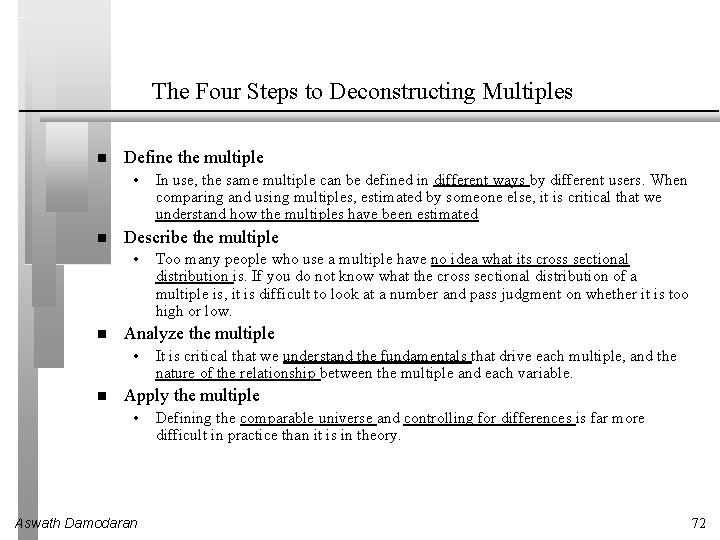
The Four Steps to Deconstructing Multiples Define the multiple • Describe the multiple • Too many people who use a multiple have no idea what its cross sectional distribution is. If you do not know what the cross sectional distribution of a multiple is, it is difficult to look at a number and pass judgment on whether it is too high or low. Analyze the multiple • In use, the same multiple can be defined in different ways by different users. When comparing and using multiples, estimated by someone else, it is critical that we understand how the multiples have been estimated It is critical that we understand the fundamentals that drive each multiple, and the nature of the relationship between the multiple and each variable. Apply the multiple • Aswath Damodaran Defining the comparable universe and controlling for differences is far more difficult in practice than it is in theory. 72

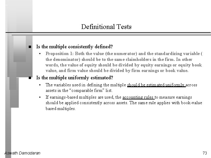
Definitional Tests Is the multiple consistently defined? • Proposition 1: Both the value (the numerator) and the standardizing variable ( the denominator) should be to the same claimholders in the firm. In other words, the value of equity should be divided by equity earnings or equity book value, and firm value should be divided by firm earnings or book value. Is the multiple uniformly estimated? • • Aswath Damodaran The variables used in defining the multiple should be estimated uniformly across assets in the “comparable firm” list. If earnings-based multiples are used, the accounting rules to measure earnings should be applied consistently across assets. The same rule applies with book-value based multiples. 73

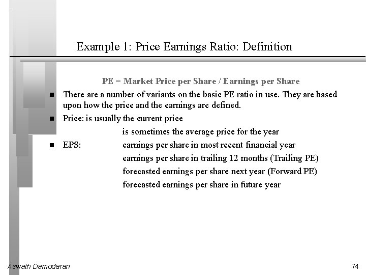
Example 1: Price Earnings Ratio: Definition PE = Market Price per Share / Earnings per Share There a number of variants on the basic PE ratio in use. They are based upon how the price and the earnings are defined. Price: is usually the current price is sometimes the average price for the year EPS: earnings per share in most recent financial year earnings per share in trailing 12 months (Trailing PE) forecasted earnings per share next year (Forward PE) forecasted earnings per share in future year Aswath Damodaran 74

Example 2: Enterprise Value /EBITDA Multiple The enterprise value to EBITDA multiple is obtained by netting cash out against debt to arrive at enterprise value and dividing by EBITDA. Why do we net out cash from firm value? What happens if a firm has cross holdings which are categorized as: • • Aswath Damodaran Minority interests? Majority active interests? 75

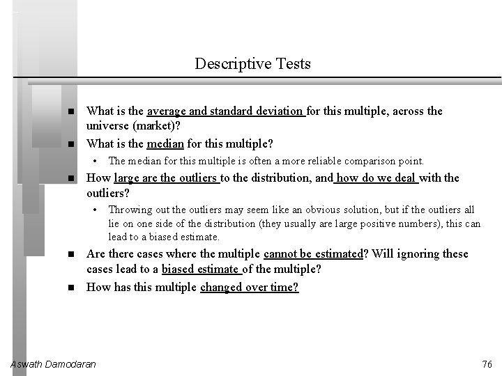
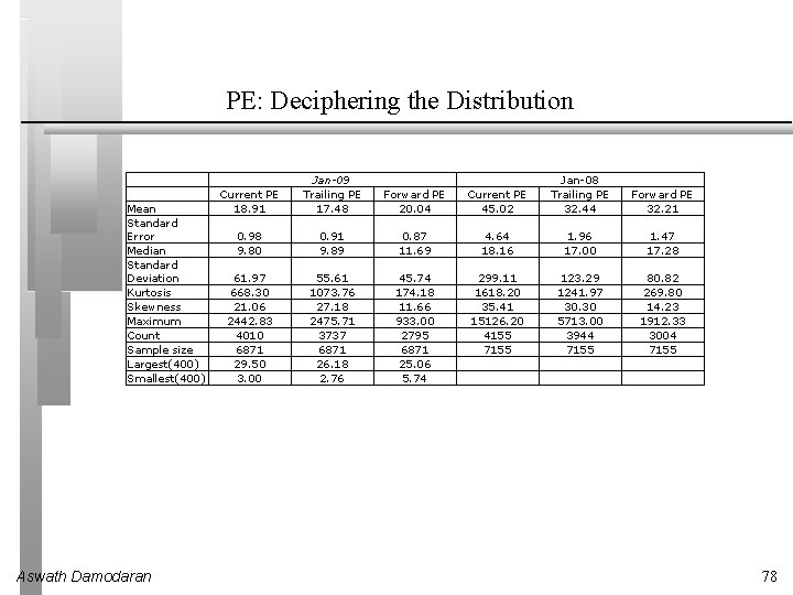
Descriptive Tests What is the average and standard deviation for this multiple, across the universe (market)? What is the median for this multiple? • How large are the outliers to the distribution, and how do we deal with the outliers? • The median for this multiple is often a more reliable comparison point. Throwing out the outliers may seem like an obvious solution, but if the outliers all lie on one side of the distribution (they usually are large positive numbers), this can lead to a biased estimate. Are there cases where the multiple cannot be estimated? Will ignoring these cases lead to a biased estimate of the multiple? How has this multiple changed over time? Aswath Damodaran 76

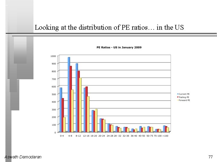
Looking at the distribution of PE ratios… in the US Aswath Damodaran 77

PE: Deciphering the Distribution Mean Standard Error Median Standard Deviation Kurtosis Skewness Maximum Count Sample size Largest(400) Smallest(400) Aswath Damodaran Current PE 18. 91 Jan-09 Trailing PE 17. 48 Forward PE 20. 04 Current PE 45. 02 Jan-08 Trailing PE 32. 44 Forward PE 32. 21 0. 98 9. 80 0. 91 9. 89 0. 87 11. 69 4. 64 18. 16 1. 96 17. 00 1. 47 17. 28 61. 97 668. 30 21. 06 2442. 83 4010 6871 29. 50 3. 00 55. 61 1073. 76 27. 18 2475. 71 3737 6871 26. 18 2. 76 45. 74 174. 18 11. 66 933. 00 2795 6871 25. 06 5. 74 299. 11 1618. 20 35. 41 15126. 20 4155 7155 123. 29 1241. 97 30. 30 5713. 00 3944 7155 80. 82 269. 80 14. 23 1912. 33 3004 7155 78

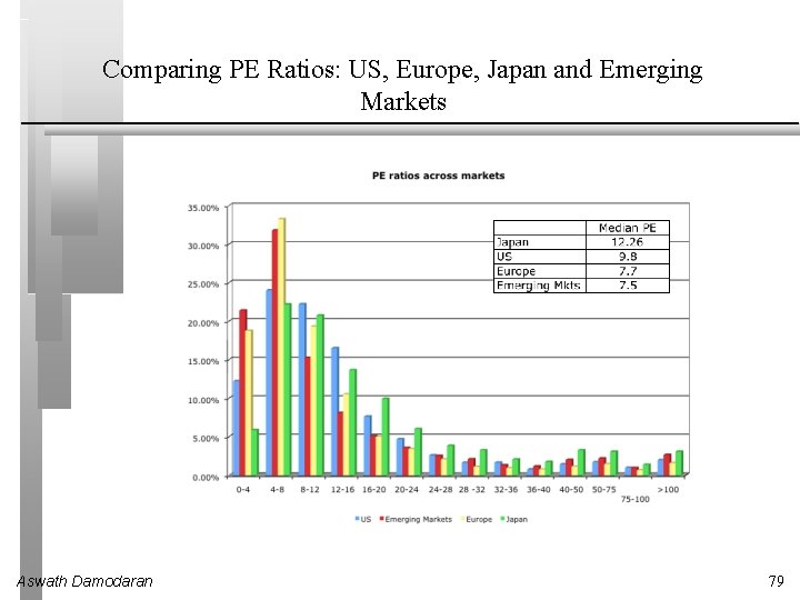
Comparing PE Ratios: US, Europe, Japan and Emerging Markets Aswath Damodaran 79

And PE ratios just for Peru… Aswath Damodaran 80

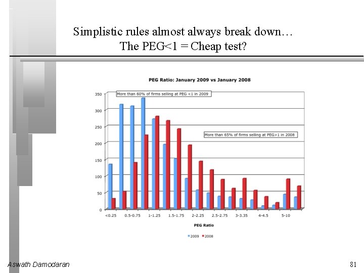
Simplistic rules almost always break down… The PEG<1 = Cheap test? Aswath Damodaran 81

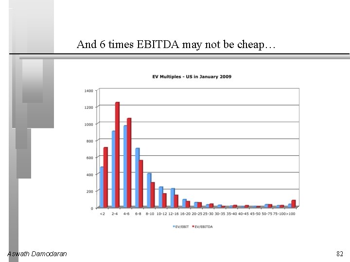
And 6 times EBITDA may not be cheap… Aswath Damodaran 82

Analytical Tests What are the fundamentals that determine and drive these multiples? • • Proposition 2: Embedded in every multiple are all of the variables that drive every discounted cash flow valuation - growth, risk and cash flow patterns. In fact, using a simple discounted cash flow model and basic algebra should yield the fundamentals that drive a multiple How do changes in these fundamentals change the multiple? • • Aswath Damodaran The relationship between a fundamental (like growth) and a multiple (such as PE) is seldom linear. For example, if firm A has twice the growth rate of firm B, it will generally not trade at twice its PE ratio Proposition 3: It is impossible to properly compare firms on a multiple, if we do not know the nature of the relationship between fundamentals and the multiple. 83

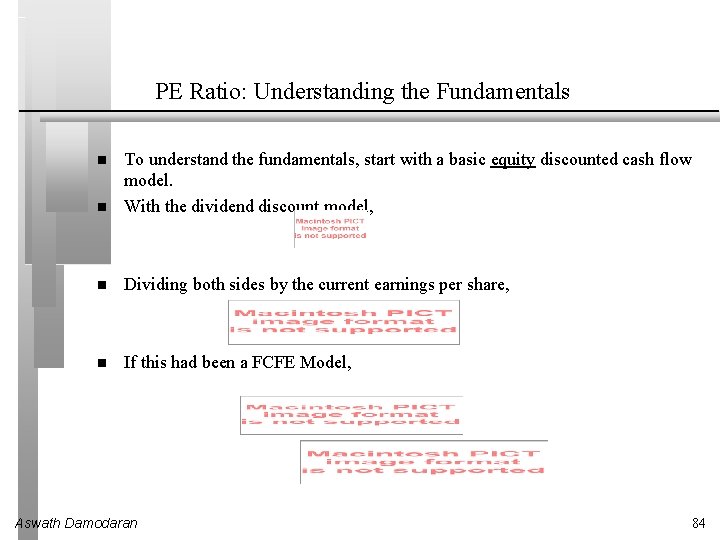
PE Ratio: Understanding the Fundamentals To understand the fundamentals, start with a basic equity discounted cash flow model. With the dividend discount model, Dividing both sides by the current earnings per share, If this had been a FCFE Model, Aswath Damodaran 84

The Determinants of Multiples… Aswath Damodaran 85

Application Tests Given the firm that we are valuing, what is a “comparable” firm? • • While traditional analysis is built on the premise that firms in the same sector are comparable firms, valuation theory would suggest that a comparable firm is one which is similar to the one being analyzed in terms of fundamentals. Proposition 4: There is no reason why a firm cannot be compared with another firm in a very different business, if the two firms have the same risk, growth and cash flow characteristics. Given the comparable firms, how do we adjust for differences across firms on the fundamentals? • Aswath Damodaran Proposition 5: It is impossible to find an exactly identical firm to the one you are valuing. 86

An Example: Comparing PE Ratios across a Sector: Telecom ADRs Aswath Damodaran 87

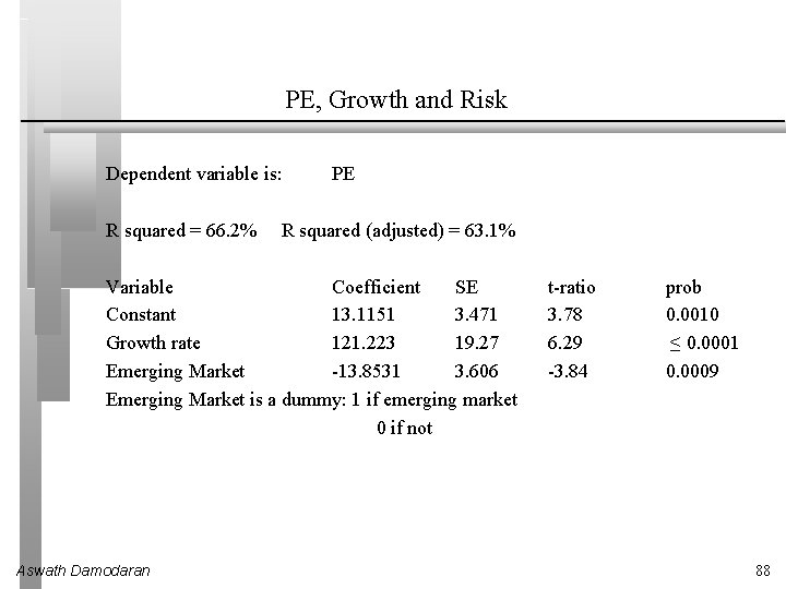
PE, Growth and Risk Dependent variable is: R squared = 66. 2% PE R squared (adjusted) = 63. 1% Variable Coefficient SE Constant 13. 1151 3. 471 Growth rate 121. 223 19. 27 Emerging Market -13. 8531 3. 606 Emerging Market is a dummy: 1 if emerging market 0 if not Aswath Damodaran t-ratio 3. 78 6. 29 -3. 84 prob 0. 0010 ≤ 0. 0001 0. 0009 88

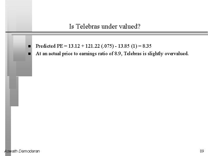
Is Telebras under valued? Predicted PE = 13. 12 + 121. 22 (. 075) - 13. 85 (1) = 8. 35 At an actual price to earnings ratio of 8. 9, Telebras is slightly overvalued. Aswath Damodaran 89

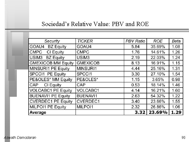
Sociedad’s Relative Value: PBV and ROE Aswath Damodaran 90

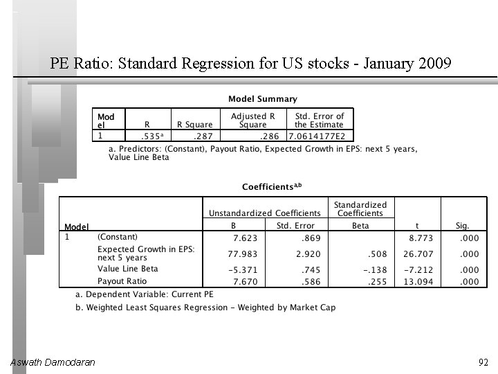
Comparisons to the entire market: Why not? In contrast to the 'comparable firm' approach, the information in the entire cross-section of firms can be used to predict PE ratios. The simplest way of summarizing this information is with a multiple regression, with the PE ratio as the dependent variable, and proxies for risk, growth and payout forming the independent variables. Aswath Damodaran 91

PE Ratio: Standard Regression for US stocks - January 2009 Aswath Damodaran 92

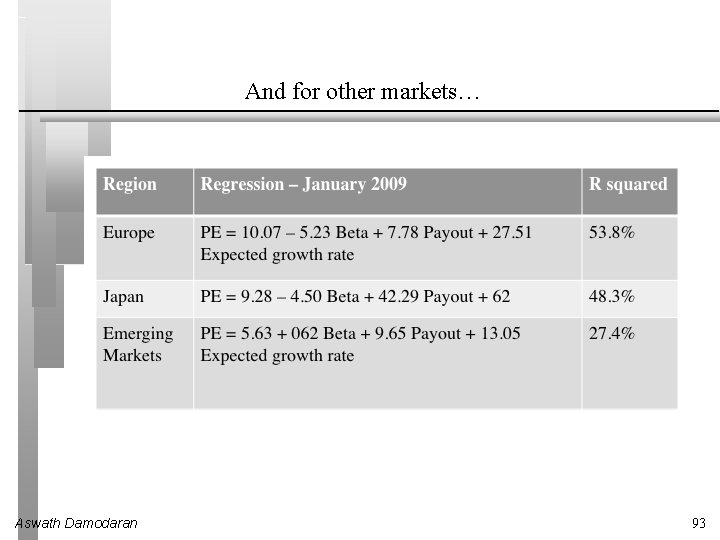
And for other markets… Aswath Damodaran 93

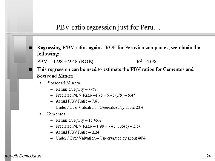
PBV ratio regression just for Peru… Regressing P/BV ratios against ROE for Peruvian companies, we obtain the following: PBV = 1. 98 + 9. 48 (ROE) R 2= 43% This regression can be used to estimate the PBV ratios for Cementos and Sociedad Minera: • Sociedad Minera – – • Cementos – – Aswath Damodaran Return on equity = 79% Predicted P/BV Ratio =1. 98 + 9. 48 (. 79) = 9. 47 Actual P/BV Ratio = 7. 61 Under / Over Valuation = Overvalued by about 23% Return on equity = 16. 45% Predicted P/BV Ratio = 1. 98 + 9. 48 (. 1645) = 3. 54 Actual P/BV Ratio = 2. 24 Under / Over Valuation = Undervalued by about 40% 94

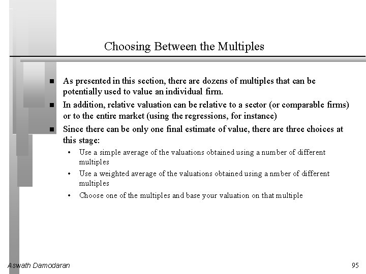
Choosing Between the Multiples As presented in this section, there are dozens of multiples that can be potentially used to value an individual firm. In addition, relative valuation can be relative to a sector (or comparable firms) or to the entire market (using the regressions, for instance) Since there can be only one final estimate of value, there are three choices at this stage: • • • Aswath Damodaran Use a simple average of the valuations obtained using a number of different multiples Use a weighted average of the valuations obtained using a nmber of different multiples Choose one of the multiples and base your valuation on that multiple 95

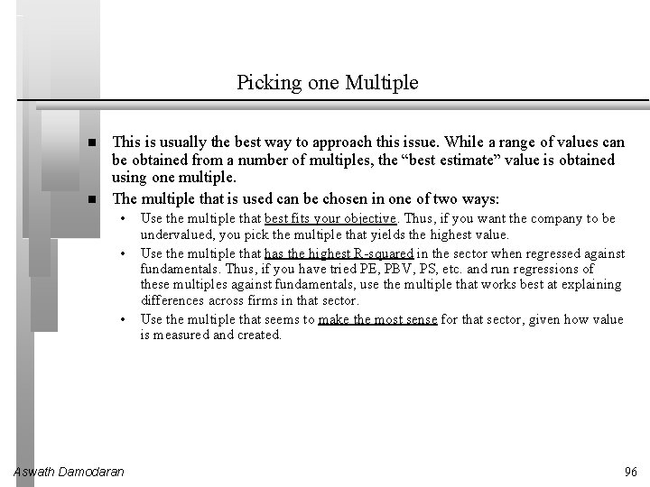
Picking one Multiple This is usually the best way to approach this issue. While a range of values can be obtained from a number of multiples, the “best estimate” value is obtained using one multiple. The multiple that is used can be chosen in one of two ways: • • • Aswath Damodaran Use the multiple that best fits your objective. Thus, if you want the company to be undervalued, you pick the multiple that yields the highest value. Use the multiple that has the highest R-squared in the sector when regressed against fundamentals. Thus, if you have tried PE, PBV, PS, etc. and run regressions of these multiples against fundamentals, use the multiple that works best at explaining differences across firms in that sector. Use the multiple that seems to make the most sense for that sector, given how value is measured and created. 96

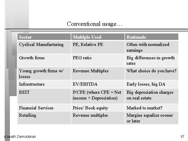
Conventional usage… Sector Multiple Used Rationale Cyclical Manufacturing PE, Relative PE Often with normalized earnings Growth firms PEG ratio Big differences in growth rates Young growth firms w/ losses Revenue Multiples What choice do you have? Infrastructure EV/EBITDA Early losses, big DA REIT P/CFE (where CFE = Net income + Depreciation) Big depreciation charges on real estate Financial Services Price/ Book equity Marked to market? Retailing Revenue multiples Margins equalize sooner or later Aswath Damodaran 97

Real Options: Fact and Fantasy Aswath Damodaran 98

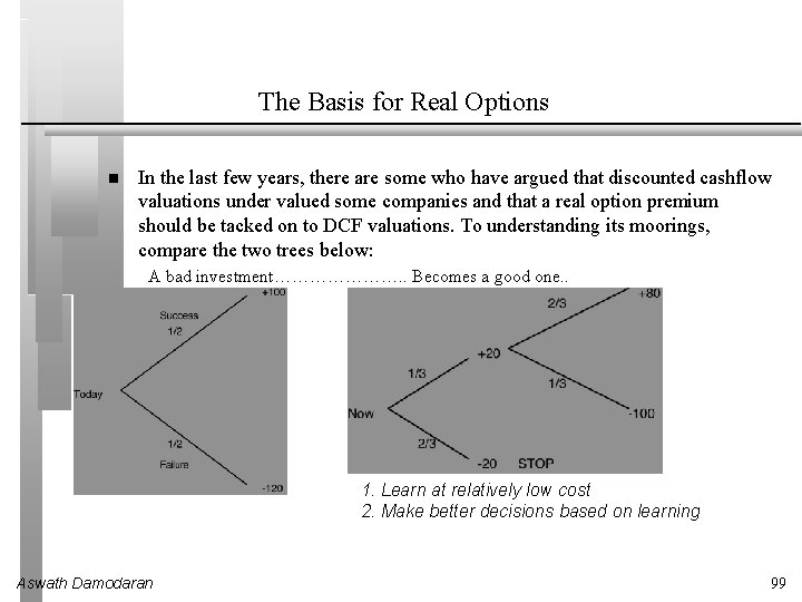
The Basis for Real Options In the last few years, there are some who have argued that discounted cashflow valuations under valued some companies and that a real option premium should be tacked on to DCF valuations. To understanding its moorings, compare the two trees below: A bad investment…………………. . Becomes a good one. . 1. Learn at relatively low cost 2. Make better decisions based on learning Aswath Damodaran 99

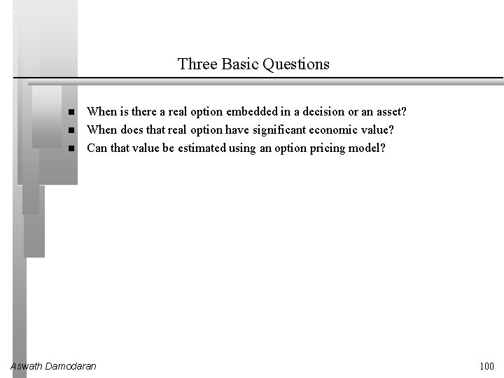
Three Basic Questions When is there a real option embedded in a decision or an asset? When does that real option have significant economic value? Can that value be estimated using an option pricing model? Aswath Damodaran 100

When is there an option embedded in an action? An option provides the holder with the right to buy or sell a specified quantity of an underlying asset at a fixed price (called a strike price or an exercise price) at or before the expiration date of the option. There has to be a clearly defined underlying asset whose value changes over time in unpredictable ways. The payoffs on this asset (real option) have to be contingent on an specified event occurring within a finite period. Aswath Damodaran 101

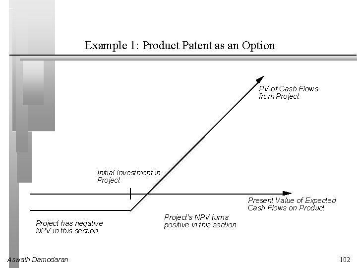
Example 1: Product Patent as an Option PV of Cash Flows from Project Initial Investment in Project Present Value of Expected Cash Flows on Product Project has negative NPV in this section Aswath Damodaran Project's NPV turns positive in this section 102

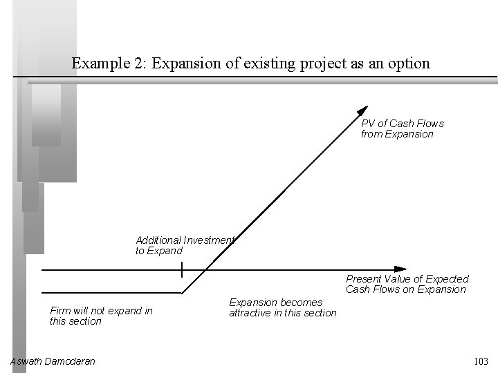
Example 2: Expansion of existing project as an option PV of Cash Flows from Expansion Additional Investment to Expand Present Value of Expected Cash Flows on Expansion Firm will not expand in this section Aswath Damodaran Expansion becomes attractive in this section 103

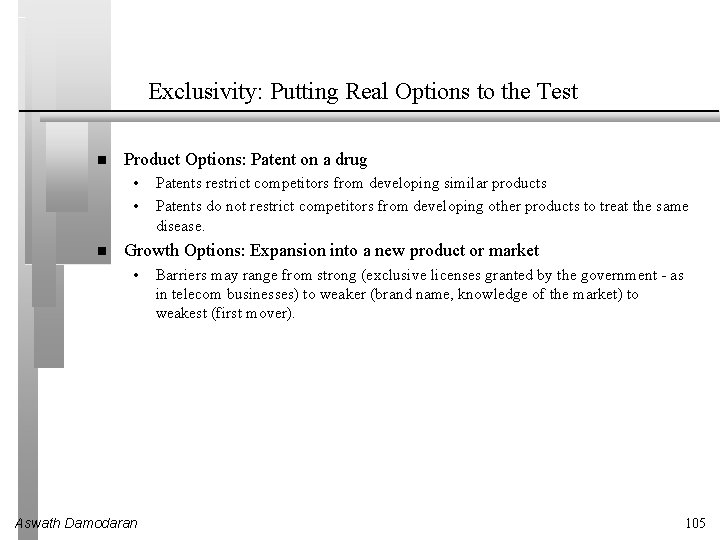
When does the option have significant economic value? For an option to have significant economic value, there has to be a restriction on competition in the event of the contingency. In a perfectly competitive product market, no contingency, no matter how positive, will generate positive net present value. At the limit, real options are most valuable when you have exclusivity - you and only you can take advantage of the contingency. They become less valuable as the barriers to competition become less steep. Aswath Damodaran 104

Exclusivity: Putting Real Options to the Test Product Options: Patent on a drug • • Patents restrict competitors from developing similar products Patents do not restrict competitors from developing other products to treat the same disease. Growth Options: Expansion into a new product or market • Aswath Damodaran Barriers may range from strong (exclusive licenses granted by the government - as in telecom businesses) to weaker (brand name, knowledge of the market) to weakest (first mover). 105

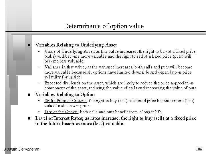
Determinants of option value Variables Relating to Underlying Asset • • • Variables Relating to Option • • Value of Underlying Asset; as this value increases, the right to buy at a fixed price (calls) will become more valuable and the right to sell at a fixed price (puts) will become less valuable. Variance in that value; as the variance increases, both calls and puts will become more valuable because all options have limited downside and depend upon price volatility for upside. Expected dividends on the asset, which are likely to reduce the price appreciation component of the asset, reducing the value of calls and increasing the value of puts. Strike Price of Options; the right to buy (sell) at a fixed price becomes more (less) valuable at a lower price. Life of the Option; both calls and puts benefit from a longer life. Level of Interest Rates; as rates increase, the right to buy (sell) at a fixed price in the future becomes more (less) valuable. Aswath Damodaran 106

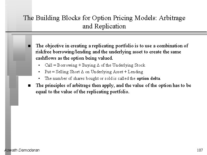
The Building Blocks for Option Pricing Models: Arbitrage and Replication The objective in creating a replicating portfolio is to use a combination of riskfree borrowing/lending and the underlying asset to create the same cashflows as the option being valued. • • • Call = Borrowing + Buying D of the Underlying Stock Put = Selling Short D on Underlying Asset + Lending The number of shares bought or sold is called the option delta. The principles of arbitrage then apply, and the value of the option has to be equal to the value of the replicating portfolio. Aswath Damodaran 107

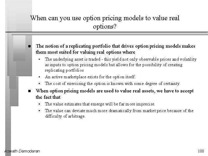
When can you use option pricing models to value real options? The notion of a replicating portfolio that drives option pricing models makes them most suited for valuing real options where • • • The underlying asset is traded - this yield not only observable prices and volatility as inputs to option pricing models but allows for the possibility of creating replicating portfolios An active marketplace exists for the option itself. The cost of exercising the option is known with some degree of certainty. When option pricing models are used to value real assets, we have to accept the fact that • • Aswath Damodaran The value estimates that emerge will be far more imprecise. The value can deviate much more dramatically from market price because of the difficulty of arbitrage. 108

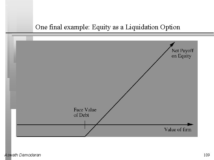
One final example: Equity as a Liquidation Option Aswath Damodaran 109

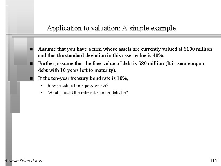
Application to valuation: A simple example Assume that you have a firm whose assets are currently valued at $100 million and that the standard deviation in this asset value is 40%. Further, assume that the face value of debt is $80 million (It is zero coupon debt with 10 years left to maturity). If the ten-year treasury bond rate is 10%, • • Aswath Damodaran how much is the equity worth? What should the interest rate on debt be? 110

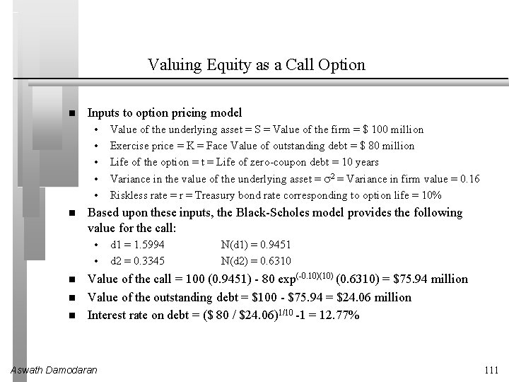
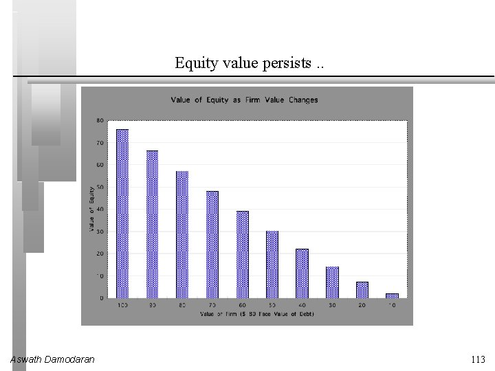
Valuing Equity as a Call Option Inputs to option pricing model • • • Based upon these inputs, the Black-Scholes model provides the following value for the call: • • Value of the underlying asset = S = Value of the firm = $ 100 million Exercise price = K = Face Value of outstanding debt = $ 80 million Life of the option = t = Life of zero-coupon debt = 10 years Variance in the value of the underlying asset = 2 = Variance in firm value = 0. 16 Riskless rate = r = Treasury bond rate corresponding to option life = 10% d 1 = 1. 5994 d 2 = 0. 3345 N(d 1) = 0. 9451 N(d 2) = 0. 6310 Value of the call = 100 (0. 9451) - 80 exp(-0. 10)(10) (0. 6310) = $75. 94 million Value of the outstanding debt = $100 - $75. 94 = $24. 06 million Interest rate on debt = ($ 80 / $24. 06)1/10 -1 = 12. 77% Aswath Damodaran 111

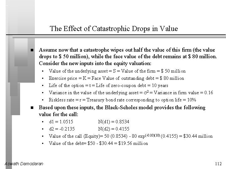
The Effect of Catastrophic Drops in Value Assume now that a catastrophe wipes out half the value of this firm (the value drops to $ 50 million), while the face value of the debt remains at $ 80 million. Consider the new inputs into the equity valuation: • • • Value of the underlying asset = S = Value of the firm = $ 50 million Exercise price = K = Face Value of outstanding debt = $ 80 million Life of the option = t = Life of zero-coupon debt = 10 years Variance in the value of the underlying asset = 2 = Variance in firm value = 0. 16 Riskless rate = r = Treasury bond rate corresponding to option life = 10% Based upon these inputs, the Black-Scholes model provides the following value for the call: • • Aswath Damodaran d 1 = 1. 0515 N(d 1) = 0. 8534 d 2 = -0. 2135 N(d 2) = 0. 4155 Value of the call (Equity)= 50 (0. 8534) - 80 exp(-0. 10)(10) (0. 4155) = $30. 44 million Value of the debt= $50 - $30. 44 = $19. 56 million 112

Equity value persists. . Aswath Damodaran 113

Back to Lemmings. . . Aswath Damodaran 114