Advanced Traffic Engineering Lecture No 4 Traffic states

Advanced Traffic Engineering Lecture No. 4 Traffic states and Phenomena by Dr. Zainab Alkaissi

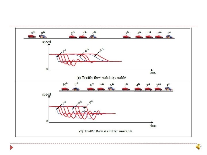
1. Stability �In traffic, we can differentiate between three levels of stability: local, platoon, and traffic. This is indicated in table below, and shown graphically in figure below:

Local stability � For local stability, one has to consider one vehicle pair, in which the second vehicle is following the leader. If the leader reduces speed, the follower needs to react. In case of local stability, he does so gracefully and relaxes into a new state. Some car following models in combination with particular parameter settings will cause the following vehicle to continuously change speeds. The following vehicle then has oscillatory speed with increasing amplitude. This is not realistic in real life traffic.

Platoon stability � For a platoon, it should be considered how a change of speed propagates through a platoon. This is called platoon stability or string stability Consider a small change in speed for the platoon leader. The following vehicle needs to react (all vehicles in the platoon are in car-following mode). Platoon stability is whether the speed disruption will grow over the vehicle number in the platoon. In platoon stable traffic, the disruption will reduce, in platoon unstable traffic, this disruption will grow. � Note that platoon stability becomes only relevant to study for locally stable traffic. For locally stable traffic, one can have platoon instability if for a single vehicle the oscillations decrease over time, but they increase over the vehicle number, as shown in figure above.

Traffic flow stability � The third type of stability is traffic flow stability. This indicates whether a traffic stream is stable. For the other types of stabilities, we have seen that stability is judged by the speed profile of another vehicle. For traffic flow stability it matters whether a change in speed of a vehicle will increase over a long time to any vehicle, even exceeding the platoon boundary. Traffic which is platoon stable is always traffic stable. The other way around, platoon unstable traffic is not always traffic unstable. It could happen that the unstable platoons are separated by gaps which are large enough to absorb disruptions. In this case, the traffic flow is stable, but the platoons are not. If the disruption propagates to other platoons, the traffic flow is unstable.

Use of stability analysis � There are mathematical tools to check analytically how disruptions are transmitted if a continuous car-following model is provided. For platoon stability this is not very realistic since all drivers drive differently. Therefore an analytical descriptions should be taken with care if used to describe traffic since one cannot assume all drivers to drive the same. � In fact, driver heterogeneity has a large impact on stability. The other way around, the stability analysis could indicate whether a car-following model is realistic. � From data, one knows that traffic is locally stable and mostly platoon unstable. Depending on the traffic flows, it can be traffic unstable or stable. For large number of vehicles, traffic is generally stable (otherwise, there would be an accident for any speed disruption).

2. Capacity drop (Phenomenon description) The capacity drop is a phenomenon that the maximum flow over a bottleneck is larger before congestion sets in than afterwards. That is, once the bottleneck is active, i. e. there is a congested state upstream of the bottleneck and no influence from bottlenecks further downstream, the traffic flow is lower. This flow is called the queue discharge rate, or sometimes the outflow capacity. � The best way to analyse this is by slated cumulative curves. Generally, the flow during congestion would be the same. That is, the queue outflow does not depend on the length of the queue. Therefore, a natural way to offset the cumulative curves is by the flow observed during discharging conditions. One would observe an increasing value before congestion sets in. � In the fundamental diagram, one would then observe a congested branch which will not reach the capacity point. Instead, one has a lower congested branch, for instance the inverse lambda fundamental diagram. The capacity drop is the difference between the free flow capacity and the queue discharge rate. This is shown in figure below. �

Illustration of the capacity drop in the fundamental diagram using real-world data.

Empirics � Capacity with congestion upstream is lower than the possible maximum flow. This capacity drop phenomenon has been empirically observed for decades. Those observations point out that the range of capacity drop, difference between the bottleneck capacity and the queue discharging rate, can vary in a wide range. Hall and Agyemang-Duah (1991) report a drop of around 6% on empirical data analysis. Cassidy and Bertini (1999) place the drop ranging from 8% to 10%. Srivastava and Geroliminis (2013) observe that the capacity falls by approximately 15% at an on-ramp bottleneck. Chung et al. (2007) present a few empirical observations of capacity drop from 3% to 18% at three active bottlenecks. Excluding the influences of light rain, they show at the same location the capacity drop can range from 8% to 18%. �

Cassidy and Rudjanakanoknad (2005) observe capacity drop ranging from 8. 3% to 14. 7%. Oh and Yeo (2012) collect empirical observations of capacity drop in nearly all previous research before 2008. The drop ranges from 3% up to 18%. The large drop of capacity reduces the performance of road network. � In most of observations, capacity drop at one bottleneck only exhibits a small day to day deviation (Chung et al. , 2007; Cassidy and Bertini, 1999). However, it is possible to observe a large difference in the capacity drop empirically at the same location. Srivastava and Geroliminis (2013) observe two different capacity drop, around 15% and 8%, at the same on-ramp bottleneck. Yuan et al. (2) observe different discharging flows at the same freeway section with a lanedrop bottleneck upstream and estimate the outflow of congestion in three-lane section ranging from 5400 vph to 6040 vph. All of these studies show that the capacity drop can be controlled and some strategies have been described to reach the goal (Chung et al. , 2007; Carlson et al. , 2010; Cassidy and Rudjanakanoknad, 2005). Those control strategies strongly rely on the relation between the congestion and the capacity drop. �

� Recent research Yuan et al. (2015 a) clearly shows this relationship with speed, see figure below. The main cause of the capacity drop is not identified yet. Some argue it is lane changing, others argue it is the limited acceleration (not instantaneous), whereas others argue it is the difference in acceleration (not all the same). This remains an active field of research, both for causes of the capacity drop and for ways to control it.

Stop-and-go wave Phenomenon description � Stop-and-go waves are a specific type of traffic jams. Generally, all traffic states at the congested branch are considered congested states. Sometimes traffic experiences short so-called stop-and-go waves. In these short traffic jams, vehicles come to (almost) a complete standstill. The duration of the queues is a few minutes. At the downstream end of the jam, there is no physical bottleneck. For many drivers, it is surprising they have been in the queue “for no obvious reason”. � The outflow of these stop-and-go waves is at the point of the queue discharge rate. Since the traffic in the jam is at almost standstill, the density in the stop-and-go wave is jam density. The speed at which the head moves, can be determined with shock wave theory. Using the fact that the wave speed is the difference in flow divided by the difference in density, we find that the head propagates backward with the wave speed (the slope of the congested branch of the fundamental diagram).

� These short jams usually start in congestion. Only if traffic is unstable, short disturbances can grow to jams. In free traffic, the spacing between platoons is usually large enough to ensure these jams do not grow. That means that upstream of the stop-and-go wave, traffic conditions are probably close to capacity. A similar traffic state upstream and downstream of the stop-and-go wave means that the upstream and downstream boundary move at the same speed. Therefore, the jam keeps it length. � Often, these type of jams occur regularly, with intervals in the order of 10 minutes. Then, the outflow of the first stop -and-go wave (queue discharge rate) is the inflow of the second one. Then, the upstream and downstream boundary must move at the same speed. �

Space-time plot of the traffic operations of the German A 5, 14 October 2001 – figure from traffic-states. com Hence, the jams move parallel in a space time figure – see also figure below.

� Since traffic in the jam is (almost) at standstill, no flow is possible. That means that the upstream boundary it must continue propagating backwards through a bottleneck – the inflow keeps at the same level and the vehicles which join the queue have no choice but join the queue keeping their desired jam spacing to their predecessor. Once the jam passes the bottleneck, the desired outflow would be the queue discharge rate of the section where the congestion is. However, the capacity of the bottleneck might be lower. � In such a case, the stop-and-go wave triggers a standing congestion, as is seen in figure below. A stop-and-go wave propagates past a botteneck near location 43 km. The outflow of the stop and go wave would be larger, but now the flow is limited. Between the stop-and-go wave and the bottleneck, a congested state occurs, of which the flow equals the flow through the bottleneck (a localised bottleneck, so at both sides the same flow). This congested state is at the fundamental diagram. For most applications where the congested branch of the fundamental diagram is considered a straight line, this congested state will lie on the line connecting the queue discharge point with the jam density.

Example of a stop-and-go wave triggering a standing queue at the A 4 motorway � The speed of the downstream boundary of the stop-and-go wave is now determined by the slope of the line connecting the “stopped” jam state with the new congestion state. Since these are all on the same line, the speed is the same, and the stop-and-go wave continues propagating.

Kerner’s Three Phase Traffic Flow Theory In the first decade of this century, the number of traffic states were debated. Kerner (2004) claimed that there would be three states (free flow, congested, and synchronised). He claimed that all other theories, using two branches of the fundamental diagram – a free flow branch and a congested branch – assumed two states. This led to a hefty scientific debate, of which the most clear objections are presented by Treiber et al. (2000) and Helbing et al. (1999). A main criticism of them is that the states are not clearly distinguished. Whereas most scientist now agree that three phase traffic flow theory is not a fully correct description of traffic flow, it includes some features which are observed in traffic. In order to discuss these features and introduce name giving for them, theory is included in the course. � This reader provides a short description for each of the states: an interested reader is referred to Kerner’s book for full information (Kerner, 2004), or the wikipedia entry on three phase traffic flow theory for more concise information. States � Kerner argues there are three different states: free flow, synchronized flow and wide moving jams. �

Free flow � In free flow traffic, vehicles are not (much) influenced by each other and can move freely. In multi-lane traffic, this means that vehicles can freely overtake. Note that as consequence, the traffic in the left lane is faster than the traffic in the right lane. The description of Kerner’s free flow state therefore has similarities with the description of the two-pipe regime in Daganzo’s theory of slugs and rabbits.

Synchronized flow � Synchronized flow is found in multi-lane traffic and is characterized by the fact that the speeds in both lanes become equal – hence the name of the state: the speeds are “synchronized”. This could be seen similar to the one-pipe regime of Daganzo. � In Kerner’s three phase traffic flow theory this is one of the congested states, the other one being wide moving jams. The characterising difference between the two is that in synchronised flow, the vehicles are moving at a (possibly high) speed, whereas in wide moving jams, they are al (almost) standstill. Kerner attributes several characteristics to the synchronized flow:

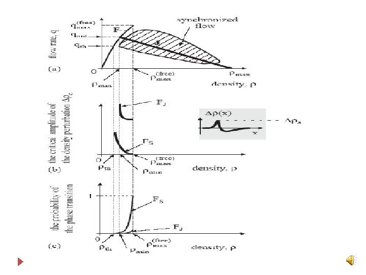
� 1. � 2. Speeds in all lanes are equal. Speeds can be high � 3. The flow can be high – possibly higher than the maximum free flow speed. Note that in this case, the “capacity” of the road is found in the synchronized flow. � 4. (Important) there is an area, rather than a line, of traffic states in the fundamental diagram. The area indicated by an “S” in figure below (a) is the area where traffic states with synchronised flow can be found. � Note that in the figure, the free flow branch (“F”) does not extend beyond the maximum flow. However, note that for a certain density, various flows are possible. The explanation by Kerner is that drivers have different equilibrium speeds, leading to different flows.

Synchronized flow

Wide moving jams A wide moving jam is most similar to what is more often called a “stop and go wave”. Stop-and-go relates to the movement an individual vehicle makes: it stops (briefly, in the order of 1 -2 minutes), and then sets off again. Kerner relates the name to the pattern (it moves in the opposite direction of the traffic stream), and “wide” is related to the width (or more accurately, it would be called length: the distance from the tail to the head) of the queue compared to the acceleration/deceleration zones surrounding the jam. The speed in the jam is (almost) 0. In the flow-density plan, the traffic state is hence found at flow (almost) 0 and jam density By consequence hence the tail moves upstream with every vehicle attaching to the jam. The head also moves upstream, since the vehicles drive off from the front. Hence the pattern of the jam moves upstream. This phenomenon is purely based on the low flow inside the jam, hence it can travel upstream for long distances (dozens of kilometers). � It can pass through areas of synchronised flow, and pass on and off ramps, see figure below: �

Observations of wide moving jams propagating through synchronised flow; figure from Kerner (2004).

Transitions � The other aspect in which Kerner’s theory deviates from the traditional view, is the transitions between the states. Kerner argues there are probabilities to go from the free flow to the synchronized flow and from synchronized flow to wide moving jams. These probabilities depend on the density, and are related to the size of a disturbance. � Let’s consider the transition from free flow to synchronized flow as an example. As the density approaches higher densities, the perturbation which is needed to move into another state, is reducing (since the propagation and amplification increases). One can draw the minimum size of an disturbance which changes the traffic state as function of the density, see next figure. Besides, one also knows with which probability these disturbances occur. Hence, one can describe with what probability a phase transition occurs, see figure below.

� Homework 1. � Can multi-anticipation improve stability? Which type and how? � � Homework 2. � Argue why traffic instability can only occur under platoon instability. � � Homework 3. � Traffic in a model is locally stable. Can the platoons be unstable? Explain why or why not. �