ADVANCED TOPICS IN DATA MINING CSE 8331 Spring

ADVANCED TOPICS IN DATA MINING CSE 8331 Spring 2010 Part I Margaret H. Dunham Department of Computer Science and Engineering Southern Methodist University 9/9/2021 1

Data Mining Outline �EMM �Stream Mining �Text Mining �Bioinformatics Mining 9/9/2021 2

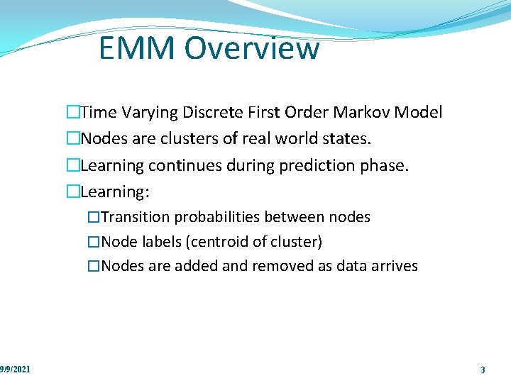
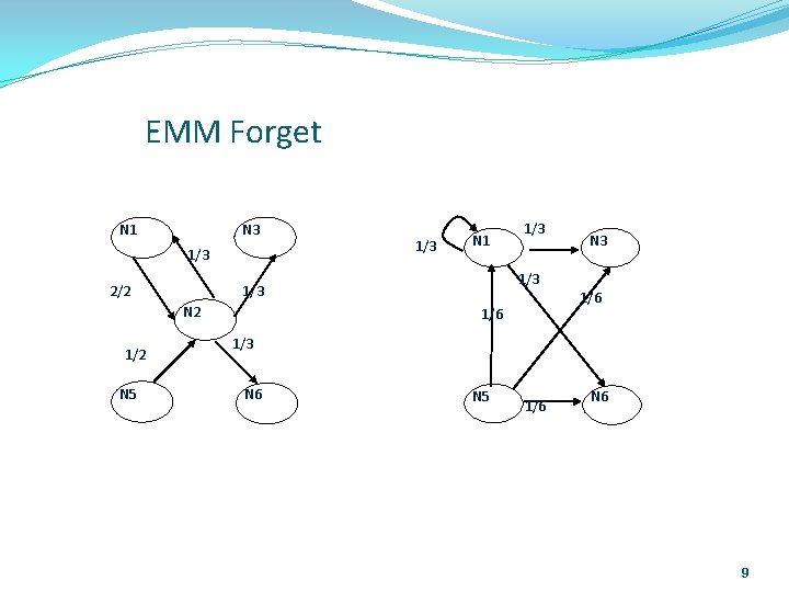
9/9/2021 EMM Overview �Time Varying Discrete First Order Markov Model �Nodes are clusters of real world states. �Learning continues during prediction phase. �Learning: �Transition probabilities between nodes �Node labels (centroid of cluster) �Nodes are added and removed as data arrives 3

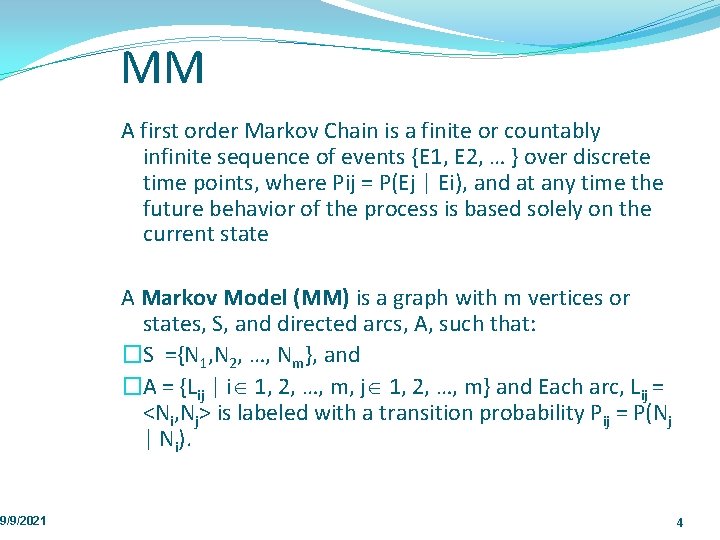
9/9/2021 MM A first order Markov Chain is a finite or countably infinite sequence of events {E 1, E 2, … } over discrete time points, where Pij = P(Ej | Ei), and at any time the future behavior of the process is based solely on the current state A Markov Model (MM) is a graph with m vertices or states, S, and directed arcs, A, such that: �S ={N 1, N 2, …, Nm}, and �A = {Lij | i 1, 2, …, m, j 1, 2, …, m} and Each arc, Lij = <Ni, Nj> is labeled with a transition probability Pij = P(Nj | Ni). 4

EMM Definition Extensible Markov Model (EMM): at any time t, EMM consists of an MC with designated current node, Nn, and algorithms to modify it, where algorithms include: �EMMCluster, which defines a technique for matching between input data at time t + 1 and existing states in the MC at time t. �EMMIncrement algorithm, which updates MC at time t + 1 given the MC at time t and clustering measure result at time t + 1. �EMMDecrement algorithm, which removes nodes from the EMM when needed. 9/9/2021 5

9/9/2021 EMM Cluster �Find closest node to incoming event. �If none “close” create new node �Labeling of cluster is centroid of members in cluster �O(n) 6

9/9/2021 EMMSim �Find closest node to incoming event. �If none “close” create new node �Labeling of cluster is centroid/medoid of members in cluster �Problem �Nearest Neighbhor O(n) �BIRCH O(lg n) � Requires second phase to recluster initial 7

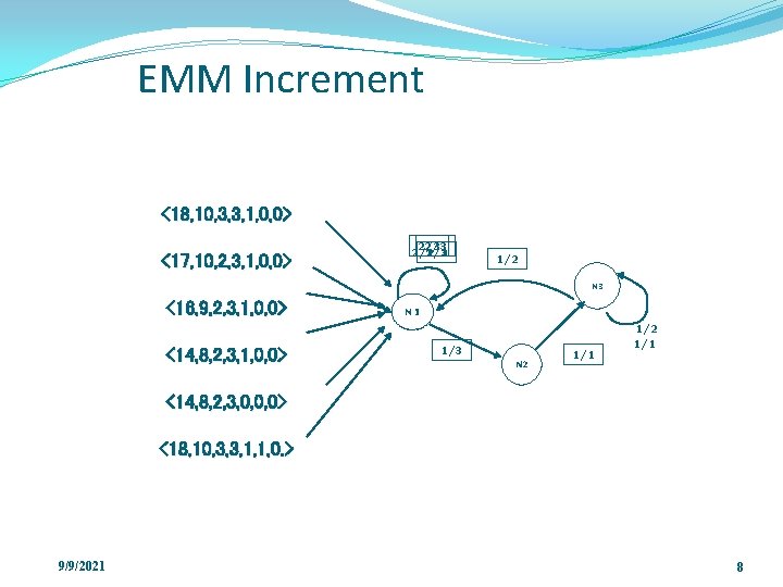
EMM Increment <18, 10, 3, 3, 1, 0, 0> <17, 10, 2, 3, 1, 0, 0> 2/3 1 1/1 2/2 1/2 2/3 1/2 N 3 <16, 9, 2, 3, 1, 0, 0> <14, 8, 2, 3, 1, 0, 0> N 1 1/3 N 2 1/1 1/2 1/1 <14, 8, 2, 3, 0, 0, 0> <18, 10, 3, 3, 1, 1, 0. > 9/9/2021 8

9/9/2021 EMM Forget N 1 N 3 1/3 2/2 N 5 1/3 N 3 1/3 N 2 1/3 N 1 1/6 1/3 N 6 N 5 1/6 N 6 9

Data Mining Outline �EMM �Stream Mining �Data Stream Overview �Data Stream Modeling �Data Stream Clustering �TRAC DS �Anomaly Detection �Text Mining �Bioinformatics Mining 9/9/2021 10

Motivation q A growing number of applications generate streams of data. Computer network monitoring data § Call detail records in telecommunications (Cisco Vo. IP 2003) § Highway transportation traffic data (Mn. Dot 2005) § Online web purchase log records (JCPenney 2003, Travelociy 2005) § Sensor network data (Ouse, Serwent 2002) § Stock exchange, transactions in retail chains, ATM operations in banks, credit card transactions. q Data mining techniques play a key role in data models in Data Stream Management System. 9/9/2021 § 11

Background Characteristics of data stream: q Data are raw q Records may at a rapid rate q High volume (possibly infinite) of continuous data q Concept drifts: Data distribution changes on the fly q Multidimensional q Temporality Stream processing restrictions: q Data modeling (synopsis) q Single pass: Each record is examined at most once q Bounded storage: Limited Memory for storing synopsis q Real time: Per record processing time must be low 9/9/2021 Haixun Wang, Jian Pei, Philip S. Yu, ICDE 2005; Keogh, ICDM’ 04 12

9/9/2021 From Sensors to Streams �Data captured and sent by a set of sensors is usually referred to as “stream data”. �Real time sequence of encoded signals which contain desired information. It is continuous, ordered (implicitly by arrival time or explicitly by timestamp or by geographic coordinates) sequence of items �Stream data is infinite the data keeps coming. 13

9/9/2021 Suppose There Were MANY Sensors �Traditional line graphs would be very difficult to read �Requirements for new visualization technique: �High level summary of data �Handle multiple sensors at once �Continuous �Temporal �Spatial 14

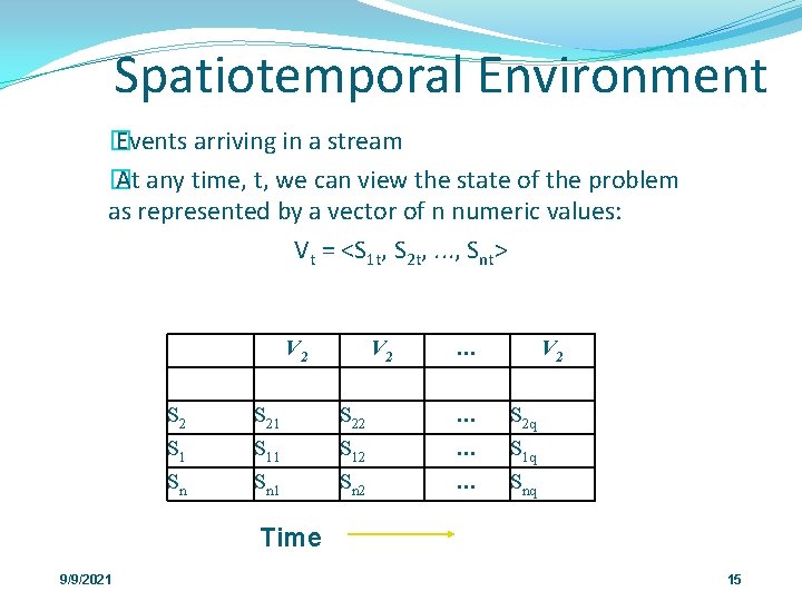
Spatiotemporal Environment � Events arriving in a stream � At any time, t, we can view the state of the problem as represented by a vector of n numeric values: Vt = <S 1 t, S 2 t, . . . , Snt> V 2 S 1 Sn S 21 S 11 Sn 1 V 2 S 22 S 12 Sn 2 … … V 2 S 2 q S 1 q Snq Time 9/9/2021 15

9/9/2021 Data Stream Management Systems (DSMS) �Software to facilitate querying and managing stream data. �Retrieve the most recent information from the stream �Data aggregation facilitates merging together multiple streams �Modeling stream data to “summarize” stream �Visualization needed to observe in real time the spatial and temporal patterns and trends hidden in the data. 16

9/9/2021 DSMS Problems �Stream Management development in state similar to that of databases prior to 1970’s �Each system/researcher looks at specific application or system �No standards concerning functionality �No standard query language �Unreasonable to expect end users will access raw data, data in the DSMS, or even data at a summarized view �Domain experts need to “see” a higher level of data 17

Data Stream Modeling 9/9/2021 �Single pass: Each record is examined at most once �Bounded storage: Limited Memory for storing synopsis �Real time: Per record processing time must be low �Summarization (Synopsis )of data �Use data NOT SAMPLE �Temporal and Spatial �Dynamic �Continuous (infinite stream) �Learn �Forget �Sublinear growth rate Clustering 18 18

9/9/2021 Problem with Markov Chains �The required structure of the MC may not be certain at the model construction time. �As the real world being modeled by the MC changes, so should the structure of the MC. �Not scalable – grows linearly as number of events. �Markov Property �Our solution: �Extensible Markov Model (EMM) �Cluster real world events �Allow Markov chain to grow and shrink dynamically 19

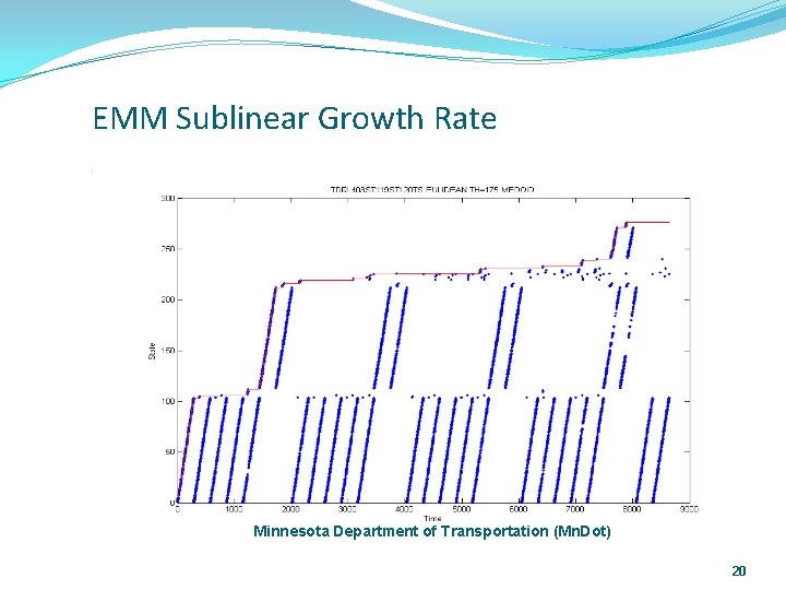
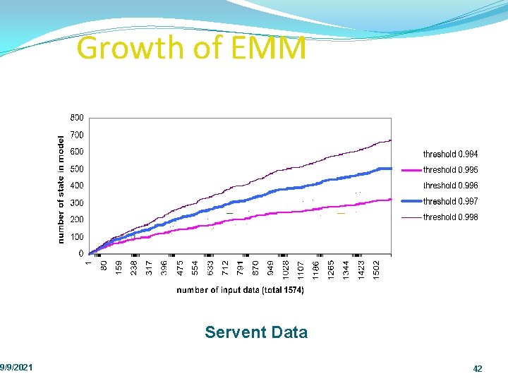
9/9/2021 EMM Sublinear Growth Rate Minnesota Department of Transportation (Mn. Dot) 20

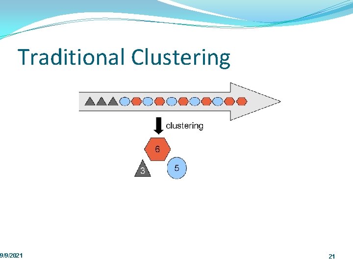
Traditional Clustering 9/9/2021 21

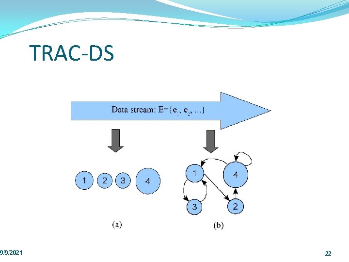
9/9/2021 TRAC DS 22

Motivation �Temporal Ordering is a major feature of stream data. �Many stream applications depend on this ordering �Prediction of future values �Anomaly (rare event) detection �Concept drift 9/9/2021 23

Stream Clustering Requirements 9/9/2021 �Dynamic updating of the clusters �Identify outliers �Barbara: �compactness �fast �incremental processing 24

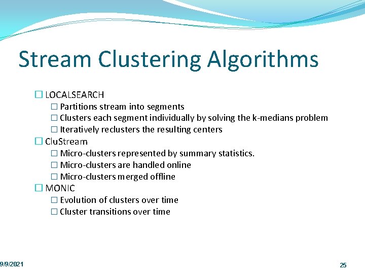
Stream Clustering Algorithms 9/9/2021 � LOCALSEARCH � Partitions stream into segments � Clusters each segment individually by solving the k medians problem � Iteratively reclusters the resulting centers � Clu. Stream � Micro clusters represented by summary statistics. � Micro clusters are handled online � Micro clusters merged offline � MONIC � Evolution of clusters over time � Cluster transitions over time 25

TRAC DS NOTE 9/9/2021 �TRAC DS is not: � Another stream clustering algorithm �TRAC DS is: �A new way of looking at clustering �Built on top of an existing clustering algorithm �TRAC DS may be used with any stream clustering algorithm 26

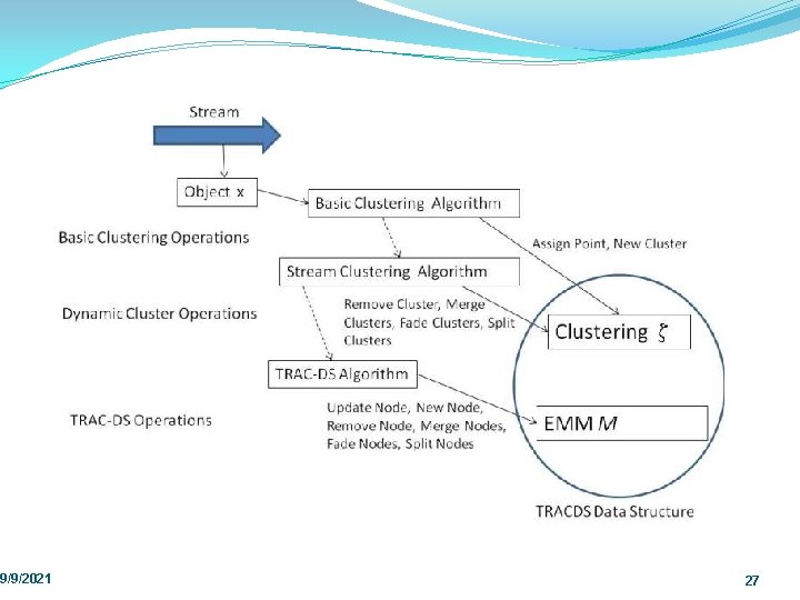
TRAC DS Overview 9/9/2021 27

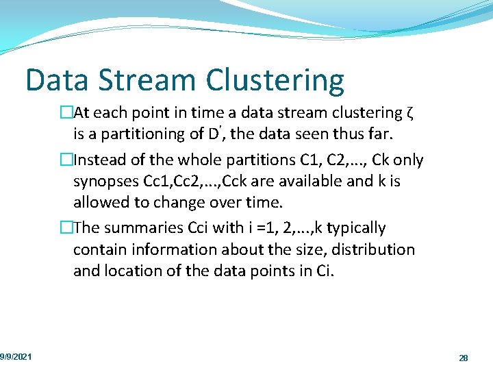
Data Stream Clustering 9/9/2021 �At each point in time a data stream clustering ζ is a partitioning of D', the data seen thus far. �Instead of the whole partitions C 1, C 2, . . . , Ck only synopses Cc 1, Cc 2, . . . , Cck are available and k is allowed to change over time. �The summaries Cci with i =1, 2, . . . , k typically contain information about the size, distribution and location of the data points in Ci. 28

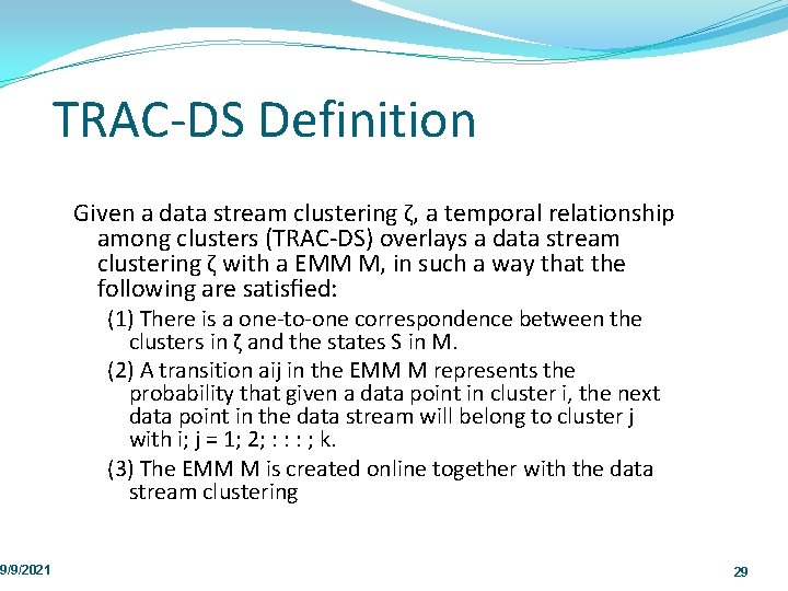
9/9/2021 TRAC DS Definition Given a data stream clustering ζ, a temporal relationship among clusters (TRAC DS) overlays a data stream clustering ζ with a EMM M, in such a way that the following are satisfied: (1) There is a one to one correspondence between the clusters in ζ and the states S in M. (2) A transition aij in the EMM M represents the probability that given a data point in cluster i, the next data point in the data stream will belong to cluster j with i; j = 1; 2; : : : ; k. (3) The EMM M is created online together with the data stream clustering 29

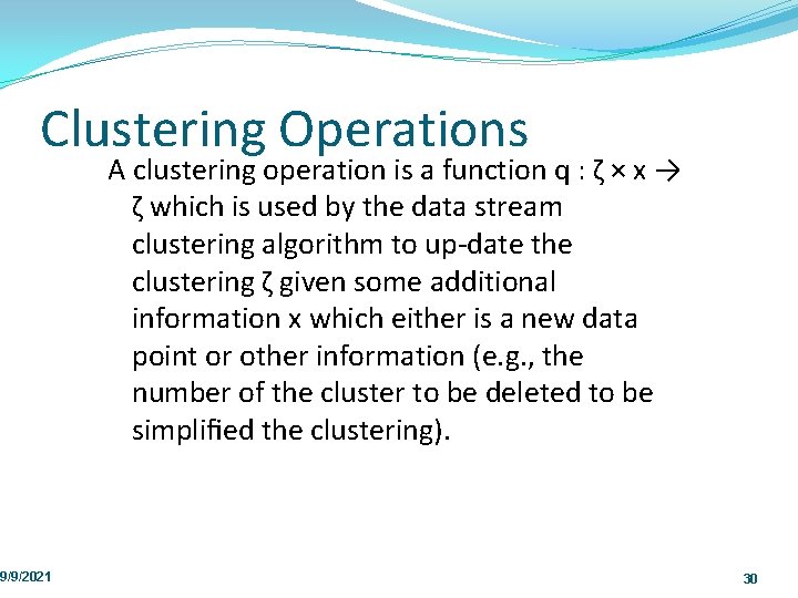
Clustering Operations 9/9/2021 A clustering operation is a function q : ζ × x → ζ which is used by the data stream clustering algorithm to up date the clustering ζ given some additional information x which either is a new data point or other information (e. g. , the number of the cluster to be deleted to be simplified the clustering). 30

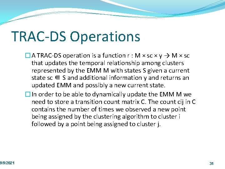
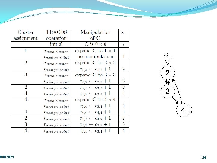
TRAC DS Operations 9/9/2021 �A TRAC DS operation is a function r : M × sc × y → M × sc that updates the temporal relationship among clusters represented by the EMM M with states S given a current state sc ∈ S and additional information y and returns an updated EMM and possibly a new current state. �In order to be able to dynamically update the EMM M we need to store a transition count matrix C. The count cij in C contains the number of times we observed a new point being assigned by the clustering algorithm to cluster i followed by a point being assigned to cluster j. 31

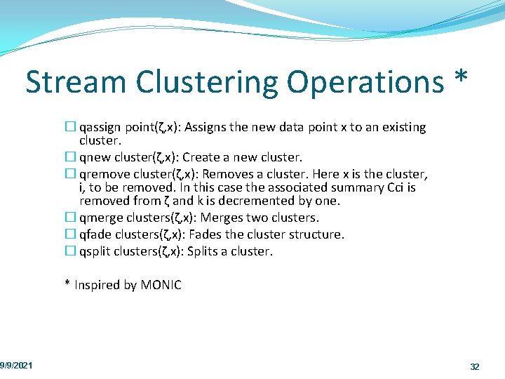
Stream Clustering Operations * 9/9/2021 � qassign point(ζ, x): Assigns the new data point x to an existing cluster. � qnew cluster(ζ, x): Create a new cluster. � qremove cluster(ζ, x): Removes a cluster. Here x is the cluster, i, to be removed. In this case the associated summary Cci is removed from ζ and k is decremented by one. � qmerge clusters(ζ, x): Merges two clusters. � qfade clusters(ζ, x): Fades the cluster structure. � qsplit clusters(ζ, x): Splits a cluster. * Inspired by MONIC 32

9/9/2021 TRAC DS Operations �rassign point(M, sc, y): Assigns the new data point to the state representing an existing cluster �rnew cluster(M, sc, y): Create a state for a new cluster. �rremove cluster(M, sc, y): Removes state. �rmerge clusters(M, sc, y): Merges two states. �rfade clusters(M, sc, y): Fades the transition probabilities using an exponential decay f(t)=2−λt �rsplit clusters(M, sc, y): Splits states. Y clustering operations. 33

TRAC DS Example 9/9/2021 34

TRAC DS Advantages �Dynamic �Flexible – �Use any Clustering Algorithm �Supports and clustering operations �Scalable �Merges Clustering & Markov Modeling 9/9/2021 35

What is Anomaly? �Event that is unusual �Event that doesn’t occur frequently �Predefined event �What is unusual? �What is deviation? 9/9/2021 36

What is Anomaly in Stream Data? �Rare Anomalous – Surprising �Out of the ordinary �Not outlier detection �No knowledge of data distribution �Data is not static �Must take temporal and spatial values into account �May be interested in sequence of events �Ex: Snow in upstate New York is not an anomaly �Snow in upstate New York in June is rare �Rare events may change over time 9/9/2021 37

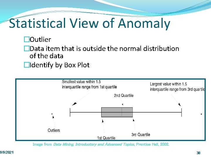
Statistical View of Anomaly 9/9/2021 �Outlier �Data item that is outside the normal distribution of the data �Identify by Box Plot Image from Data Mining, Introductory and Advanced Topics, Prentice Hall, 2002. 38

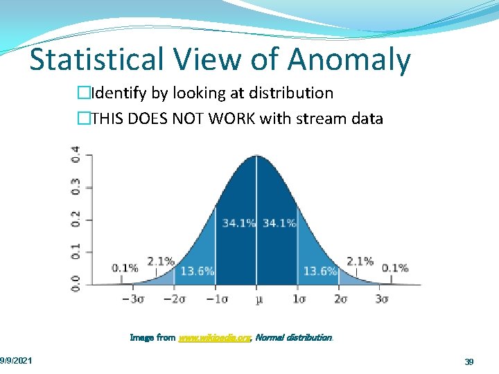
Statistical View of Anomaly 9/9/2021 �Identify by looking at distribution �THIS DOES NOT WORK with stream data Image from www. wikipedia. org, Normal distribution. 39

Data Mining View of Anomaly 9/9/2021 �Classification Problem �Build classifier from training data �Problem is that training data shows what is NOT an anomaly �Thus an anomaly is anything that is not viewed as normal by the classification technique �MUST build dynamic classifier �Identify anomalous behavior �Signatures of what anomalous behavior looks like �Input data is identified as anomaly if it is similar enough to one of these signatures �Mixed – Classification and Signature 40

9/9/2021 EMM Advantages �Dynamic �Adaptable �Use of clustering �Learns rare event �Scalable: �Growth of EMM is not linear on size of data. �Hierarchical feature of EMM �Creation/evaluation quasi real time �Distributed / Hierarchical extensions 41

9/9/2021 Growth of EMM Servent Data 42

TRAC DS Approach to Detect Anomalies 9/9/2021 �By learning what is normal, the model can predict what is not �Normal is based on likelihood of occurrence �Use TRAC DS to build clusters and behavior between clusters �We view a rare event as: �Unusual event �Transition between events states which does not frequently occur. �Continue learning 43

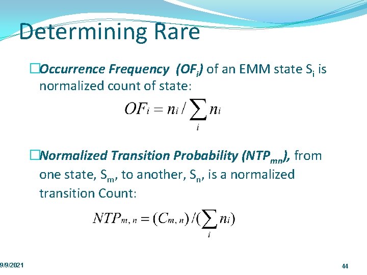
Determining Rare 9/9/2021 �Occurrence Frequency (OFi) of an EMM state Si is normalized count of state: �Normalized Transition Probability (NTPmn), from one state, Sm, to another, Sn, is a normalized transition Count: 44

9/9/2021 EMMRare �EMMRare algorithm indicates if the current input event is rare. Using a threshold occurrence percentage, the input event is determined to be rare if either of the following occurs: �The frequency of the node at time t+1 is below this threshold �The updated transition probability of the MC transition from node at time t to the node at t+1 is below the threshold 45