Advanced Topics in Data Analysis Shai Carmi Introduction

Advanced Topics in Data Analysis Shai Carmi

Introduction to machine learning • Basic concepts • Supervised learning: classifiers o o K-nearest neighbors Logistic regression Measuring accuracy The perceptron and neural networks • Unsupervised learning: clustering and dimension reduction

Unsupervised learning • Clustering: introduction and k-means • Hierarchical clustering • Dimension reduction

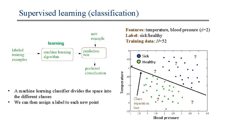
Supervised learning (classification) Features: temperature, blood pressure (d=2) Label: sick/healthy Training data: N=52 learning Sick Healthy ? ? Temperature • A machine learning classifier divides the space into the different classes • We can then assign a label to each new point ? Class separation line ? Blood pressure ?

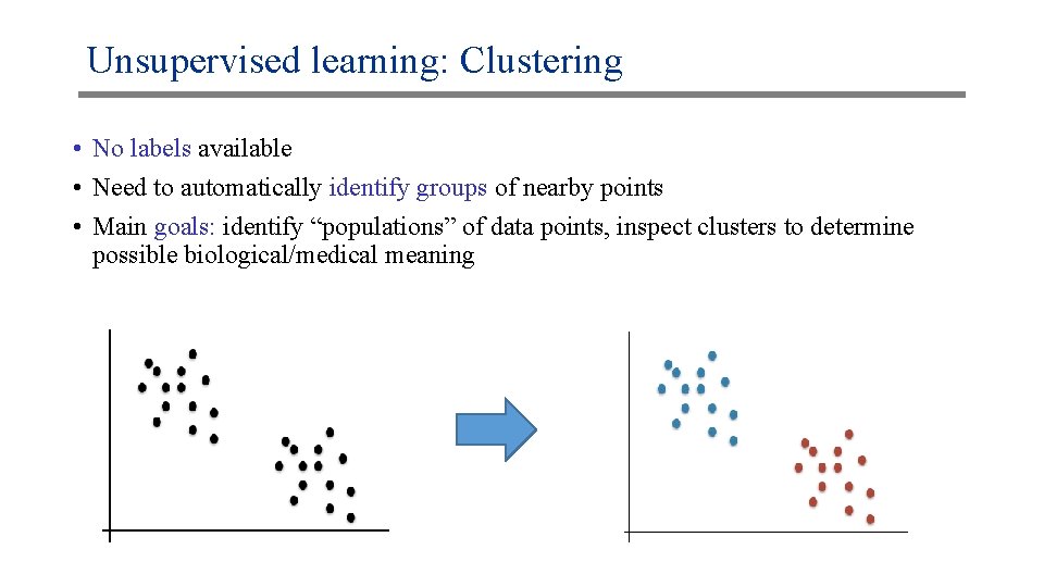
Unsupervised learning: Clustering • No labels available • Need to automatically identify groups of nearby points • Main goals: identify “populations” of data points, inspect clusters to determine possible biological/medical meaning

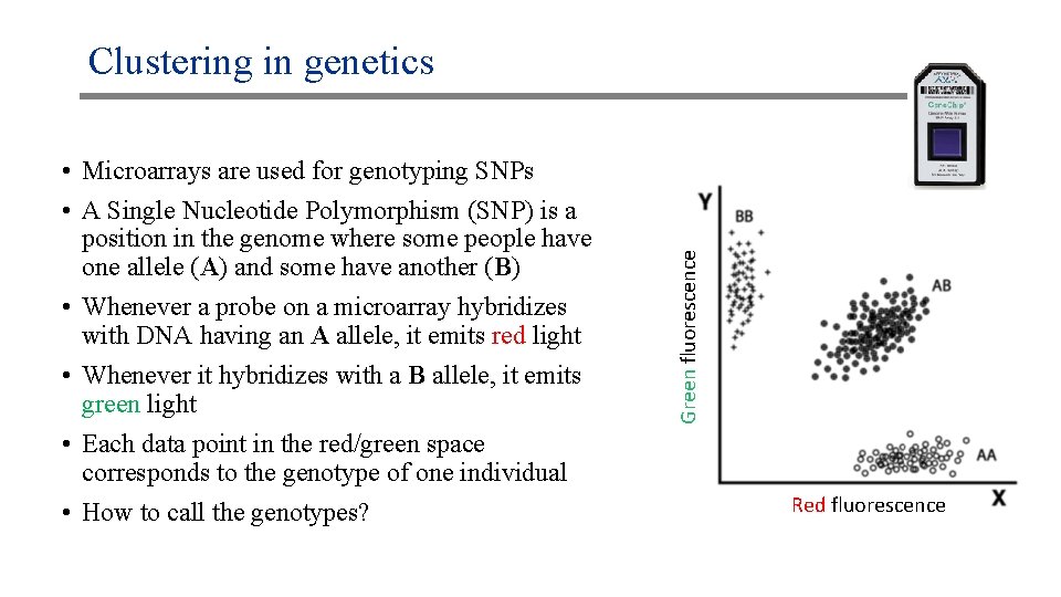
• Microarrays are used for genotyping SNPs • A Single Nucleotide Polymorphism (SNP) is a position in the genome where some people have one allele (A) and some have another (B) • Whenever a probe on a microarray hybridizes with DNA having an A allele, it emits red light • Whenever it hybridizes with a B allele, it emits green light • Each data point in the red/green space corresponds to the genotype of one individual • How to call the genotypes? Green fluorescence Clustering in genetics Red fluorescence

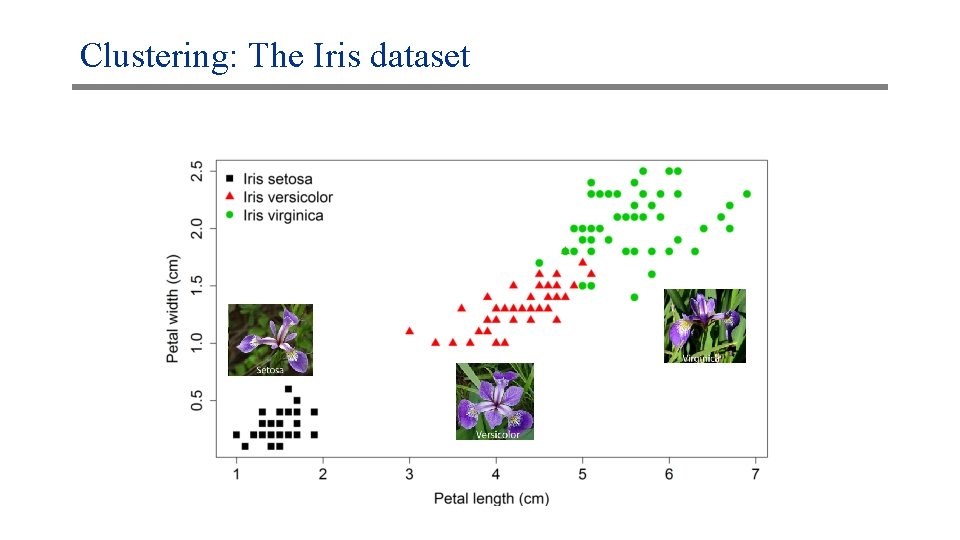
Clustering: The Iris dataset

Clustering: Motivation • An exploratory analysis for understanding the data • Sometimes the groups are known and we can guess the labels from the clusters • Find sub-groups in data that may be heterogeneous o o Subjects of medical study Subtypes of cancer tissues • Information on cluster locations can be useful

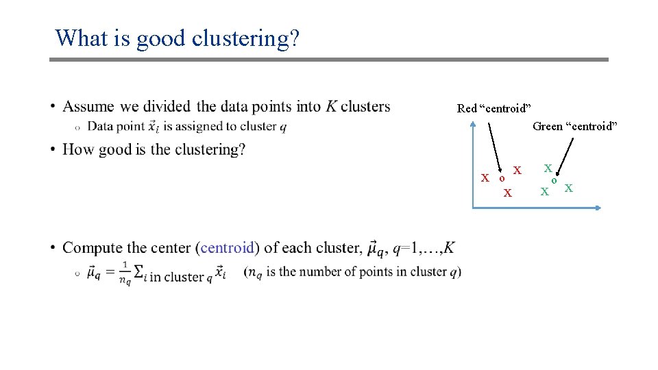
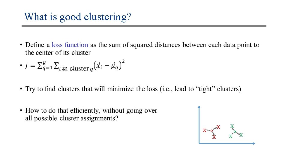
What is good clustering? • Red “centroid” Green “centroid” x o x x

What is good clustering? • x o x x

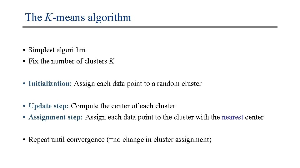
The K-means algorithm • Simplest algorithm • Fix the number of clusters K • Initialization: Assign each data point to a random cluster • Update step: Compute the center of each cluster • Assignment step: Assign each data point to the cluster with the nearest center • Repeat until convergence (=no change in cluster assignment)

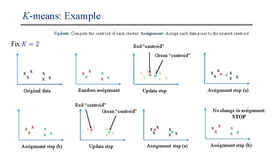
K-means: Example Update: Compute the centroid of each cluster; Assignment: Assign each data point to the nearest centroid Red “centroid” Green “centroid” x x x Original data x x x Random assignment x xo o x x x x Assignment step (a) Update step Red “centroid” Green “centroid” x x x Assignment step (b) x ox x x o x x Update step No change in assignment: STOP x ox x x o x x Assignment step (a) x x x Assignment step (b)

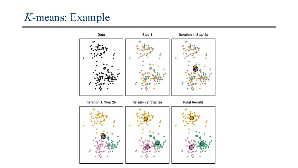
K-means: Example

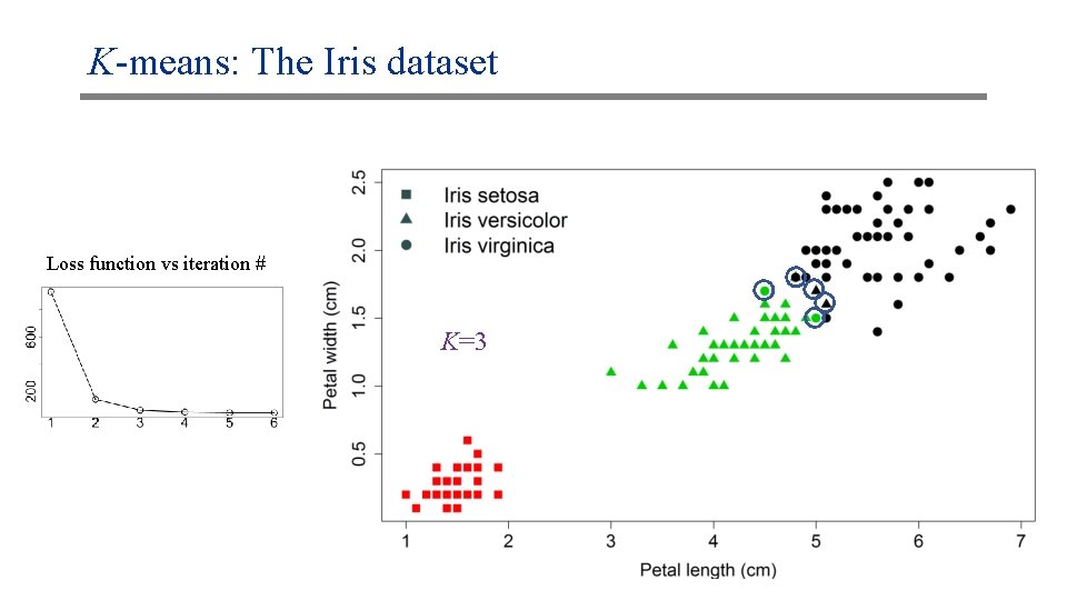
K-means: The Iris dataset Loss function vs iteration # K=3

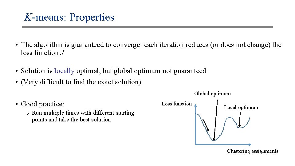
K-means: Properties • The algorithm is guaranteed to converge: each iteration reduces (or does not change) the loss function J • Solution is locally optimal, but global optimum not guaranteed • (Very difficult to find the exact solution) Global optimum • Good practice: o Run multiple times with different starting points and take the best solution Loss function Local optimum Clustering assignments

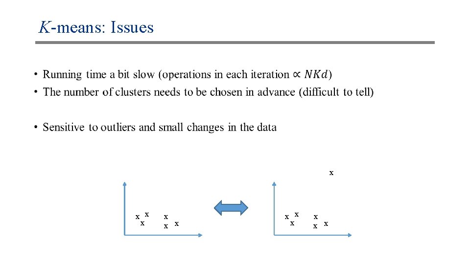
K-means: Issues • x x x x

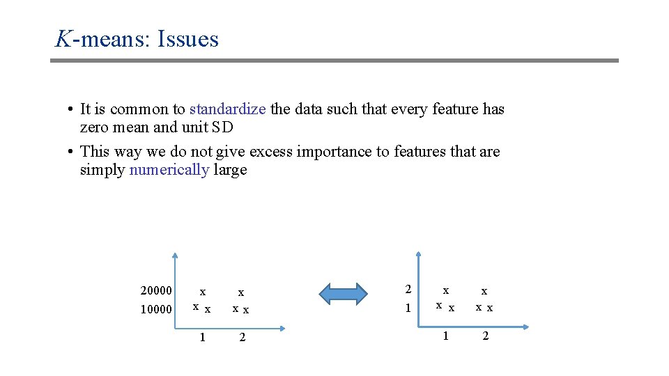
K-means: Issues • It is common to standardize the data such that every feature has zero mean and unit SD • This way we do not give excess importance to features that are simply numerically large 20000 10000 x x xx 1 2 2 1 x x xx 1 2

K-means: Variants • K-means forces each point to be assigned to exactly one cluster • It will be useful to give the probability of each point to be assigned to each of the possible clusters • The Expectation-Maximization algorithm is able to compute such probabilities (very important method but complicated for this class)

Unsupervised learning • Clustering: introduction and k-means • Hierarchical clustering • Dimension reduction

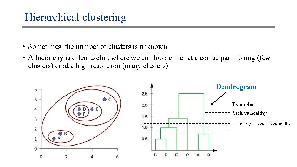
Hierarchical clustering • Sometimes, the number of clusters is unknown • A hierarchy is often useful, where we can look either at a coarse partitioning (few clusters) or at a high resolution (many clusters) Dendrogram Examples: Sick vs healthy Extremely sick vs healthy

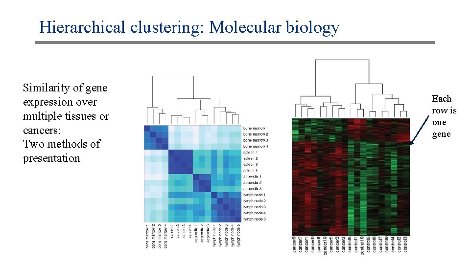
Hierarchical clustering: Molecular biology Similarity of gene expression over multiple tissues or cancers: Two methods of presentation Each row is one gene

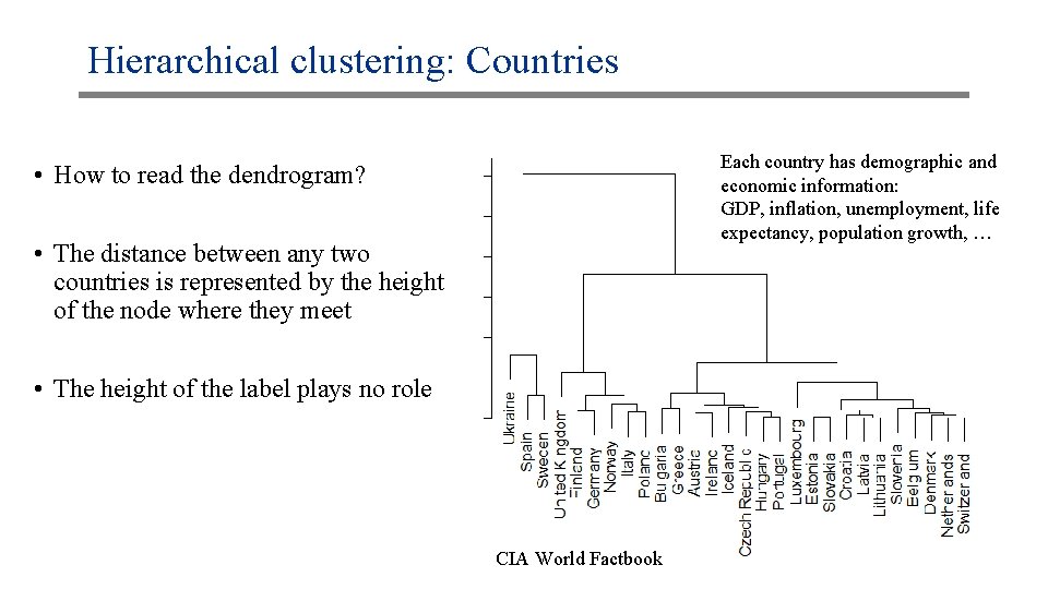
Hierarchical clustering: Countries Each country has demographic and economic information: GDP, inflation, unemployment, life expectancy, population growth, … • How to read the dendrogram? • The distance between any two countries is represented by the height of the node where they meet • The height of the label plays no role CIA World Factbook

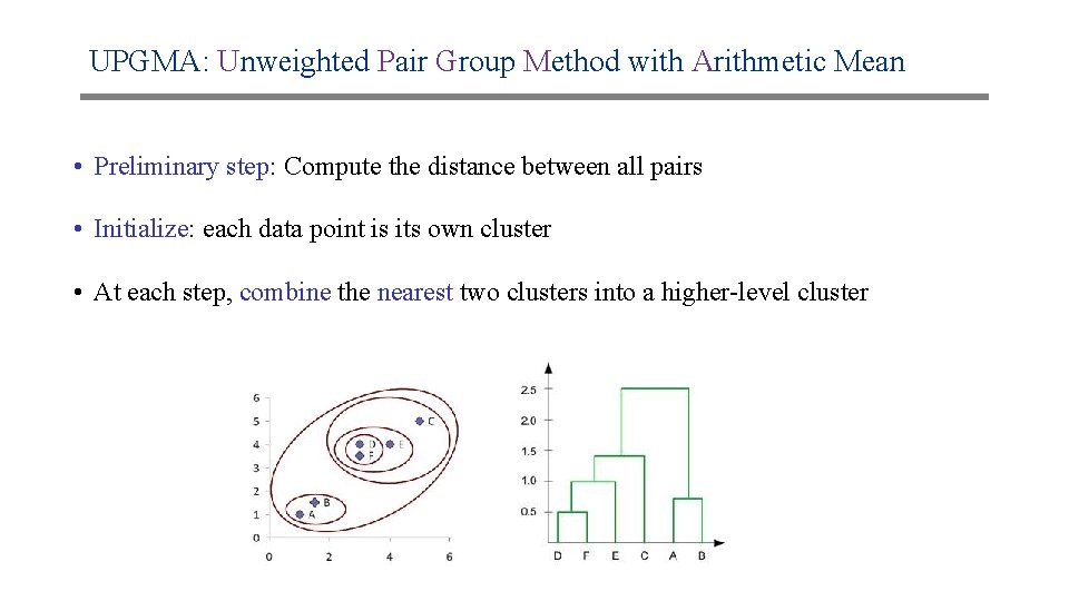
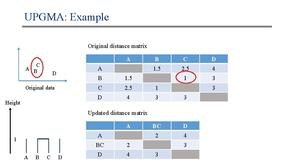
UPGMA: Unweighted Pair Group Method with Arithmetic Mean • Preliminary step: Compute the distance between all pairs • Initialize: each data point is its own cluster • At each step, combine the nearest two clusters into a higher-level cluster

UPGMA: Nearest clusters • How do we know which two clusters are the nearest? • We need a measure of distance between clusters • Definition: The distance between two clusters is the average distance between all pairs of data points in those clusters • Other choices also possible

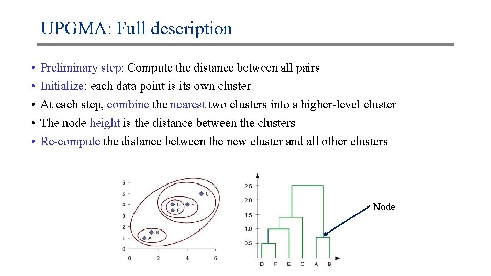
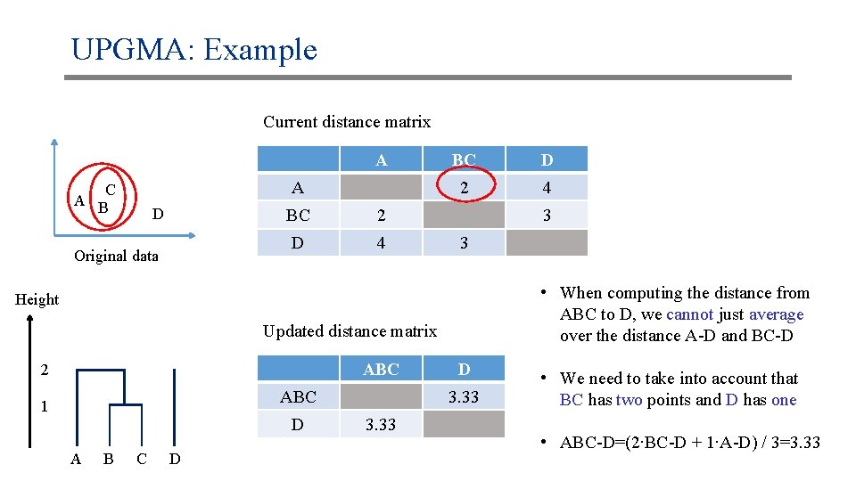
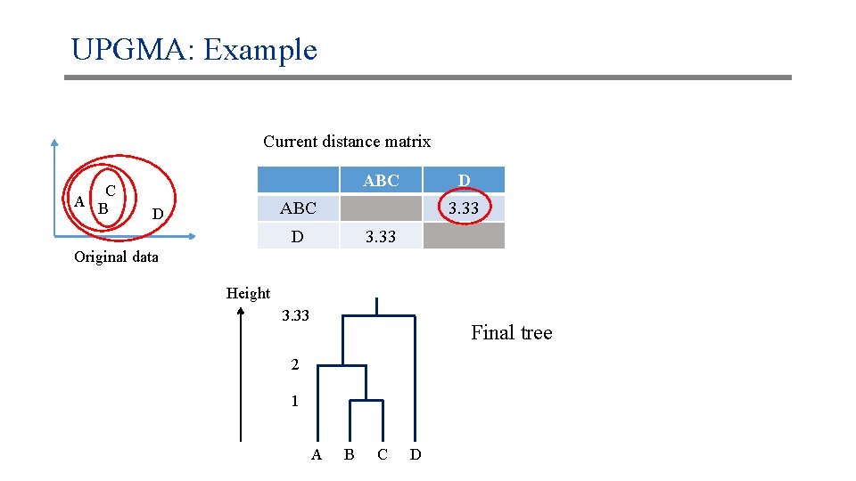
UPGMA: Full description • • • Preliminary step: Compute the distance between all pairs Initialize: each data point is its own cluster At each step, combine the nearest two clusters into a higher-level cluster The node height is the distance between the clusters Re-compute the distance between the new cluster and all other clusters Node

UPGMA: Example Original distance matrix A C A B A D Original data Height B C D 1. 5 2. 5 4 1 3 B 1. 5 C 2. 5 1 D 4 3 3 BC D 2 4 3 Updated distance matrix A A 1 A B C D BC 2 D 4 3 3

UPGMA: Example Current distance matrix A A C A B D Original data BC 2 D 4 BC D 2 4 3 3 • When computing the distance from ABC to D, we cannot just average over the distance A-D and BC-D Height Updated distance matrix ABC 2 ABC 1 D A B C D D 3. 33 • We need to take into account that BC has two points and D has one • ABC-D=(2∙BC-D + 1∙A-D) / 3=3. 33

UPGMA: Example Current distance matrix C A B ABC D 3. 33 Original data Height 3. 33 Final tree 2 1 A B C D

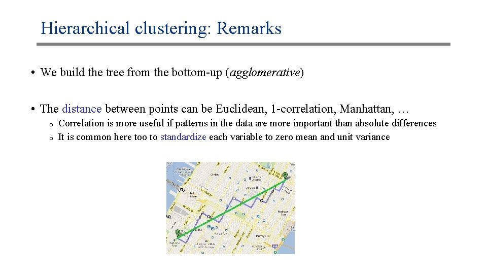
Hierarchical clustering: Remarks • We build the tree from the bottom-up (agglomerative) • The distance between points can be Euclidean, 1 -correlation, Manhattan, … o o Correlation is more useful if patterns in the data are more important than absolute differences It is common here too to standardize each variable to zero mean and unit variance

Hierarchical clustering: Remarks • Beyond “Average”, other choices are available for the way distances are calculated between clusters • Most popular are Complete (max distance), Single (min distance) • It is common to consider multiple choices for the clustering parameters • And to compare the clustering on different subsets of the data

Unsupervised learning • Clustering: introduction and k-means • Hierarchical clustering • Dimension reduction

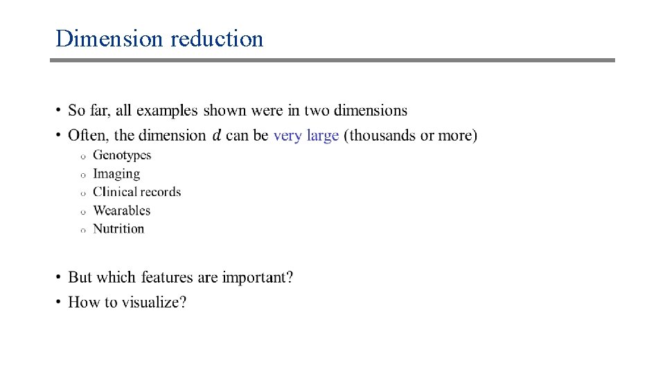
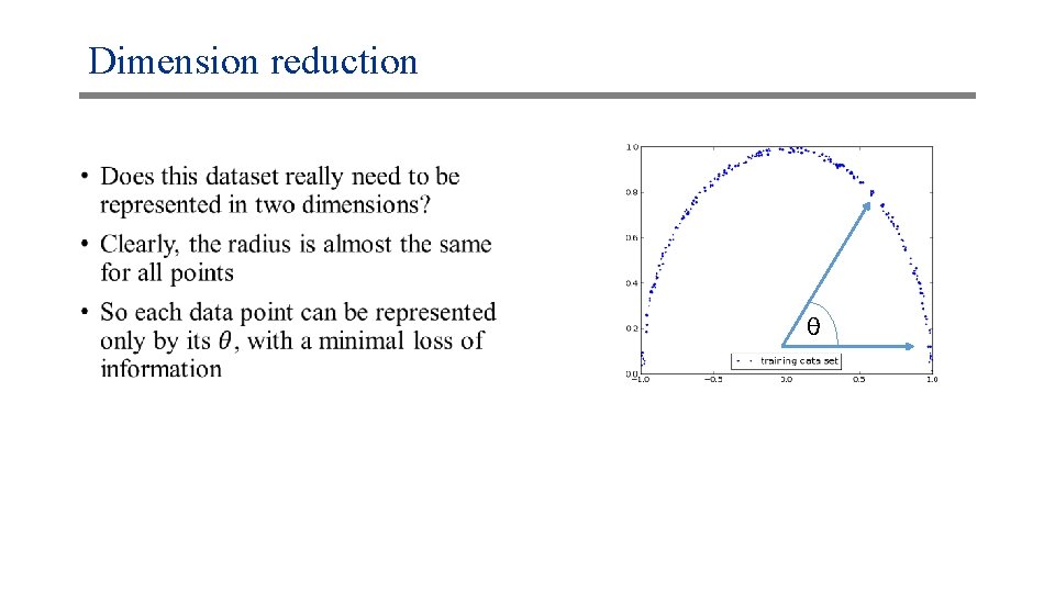
Dimension reduction •

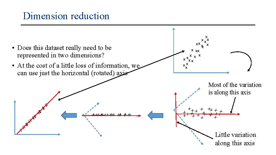
Dimension reduction • Does this dataset really need to be represented in two dimensions? • At the cost of a little loss of information, we can use just the horizontal (rotated) axis x x xx xx x x xx Most of the variation is along this axis xx xx xx x x xx xx xx x xx Little variation along this axis

Dimension reduction • θ

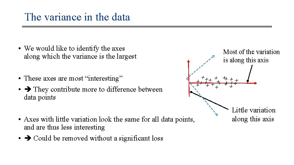
The variance in the data • We would like to identify the axes along which the variance is the largest xx xx xx x x xx • These axes are most “interesting” • They contribute more to difference between data points Most of the variation is along this axis • Axes with little variation look the same for all data points, and are thus less interesting • Could be removed without a significant loss Little variation along this axis

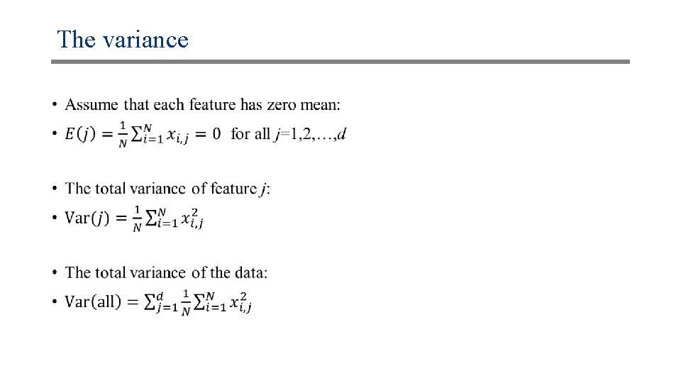
The variance •

How to reduce the dimension? • We would like to identify axes along which the data is most variable • We could then keep them and remove the other axes • The most important and popular method of dimension reduction is Principal Component Analysis (PCA)

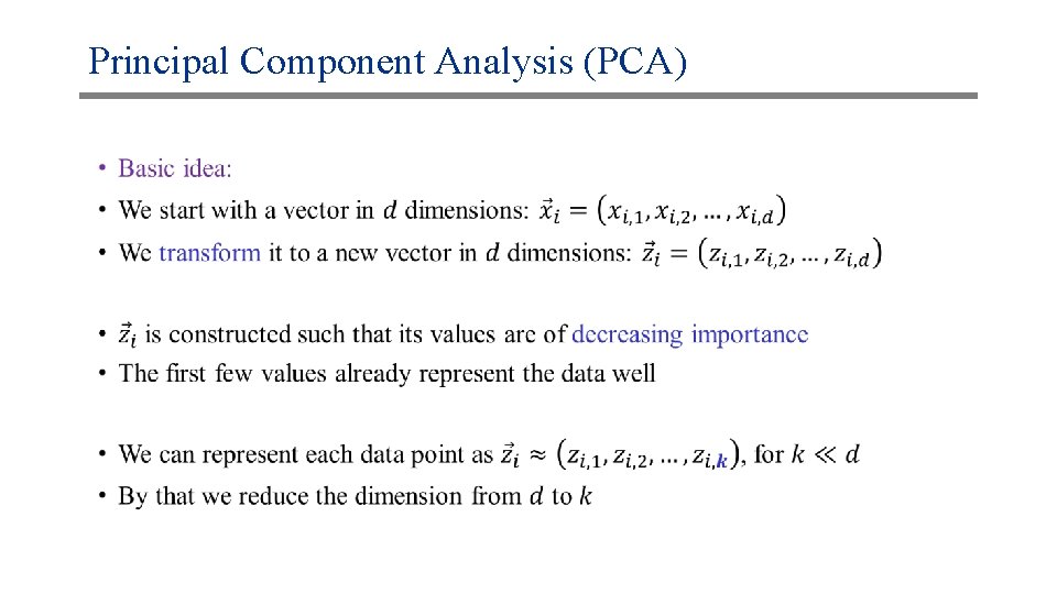
Principal Component Analysis (PCA) •

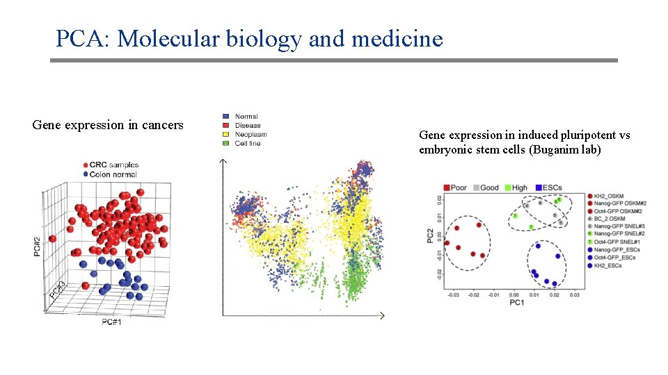
PCA: Molecular biology and medicine Gene expression in cancers Gene expression in induced pluripotent vs embryonic stem cells (Buganim lab)

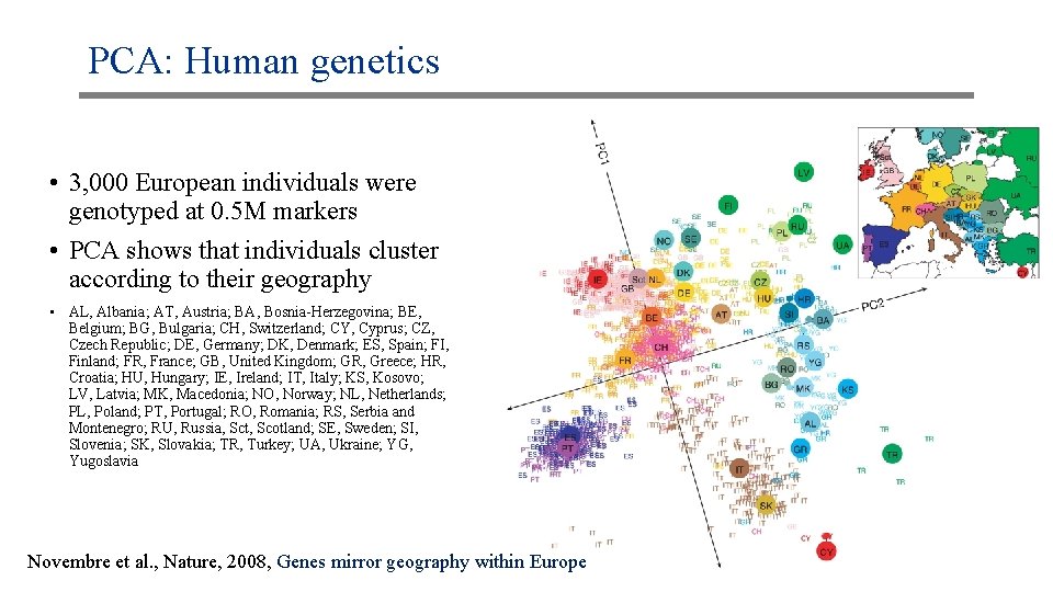
PCA: Human genetics • 3, 000 European individuals were genotyped at 0. 5 M markers • PCA shows that individuals cluster according to their geography • AL, Albania; AT, Austria; BA, Bosnia-Herzegovina; BE, Belgium; BG, Bulgaria; CH, Switzerland; CY, Cyprus; CZ, Czech Republic; DE, Germany; DK, Denmark; ES, Spain; FI, Finland; FR, France; GB, United Kingdom; GR, Greece; HR, Croatia; HU, Hungary; IE, Ireland; IT, Italy; KS, Kosovo; LV, Latvia; MK, Macedonia; NO, Norway; NL, Netherlands; PL, Poland; PT, Portugal; RO, Romania; RS, Serbia and Montenegro; RU, Russia, Sct, Scotland; SE, Sweden; SI, Slovenia; SK, Slovakia; TR, Turkey; UA, Ukraine; YG, Yugoslavia Novembre et al. , Nature, 2008, Genes mirror geography within Europe

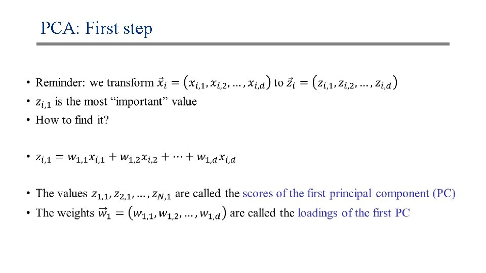
PCA: First step •

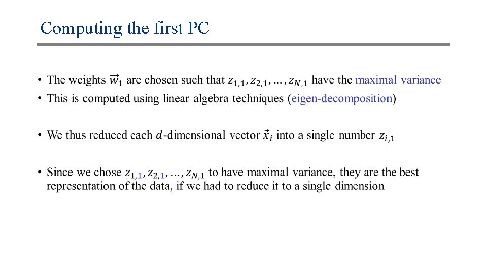
Computing the first PC •

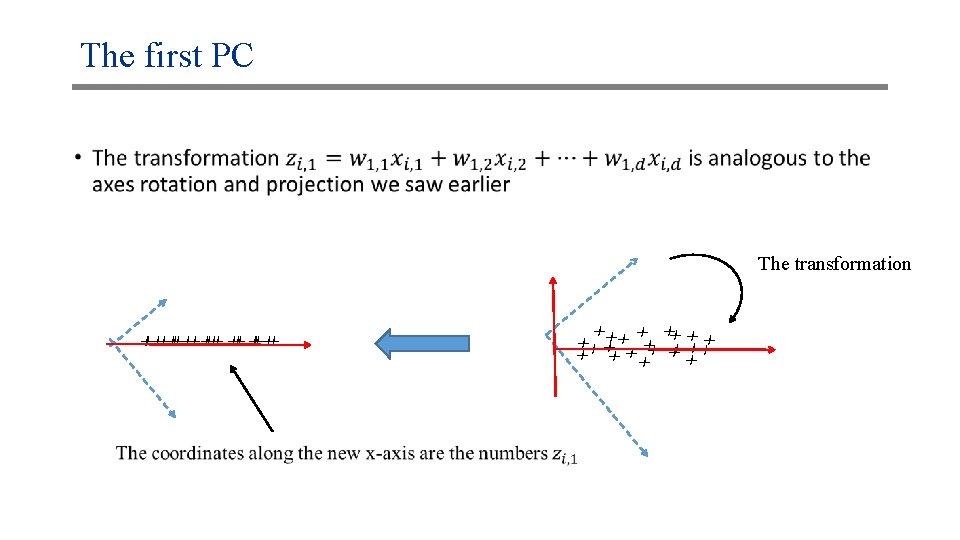
The first PC • The transformation xx xx xx x x xx xx xx x

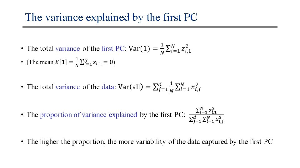
The variance explained by the first PC •

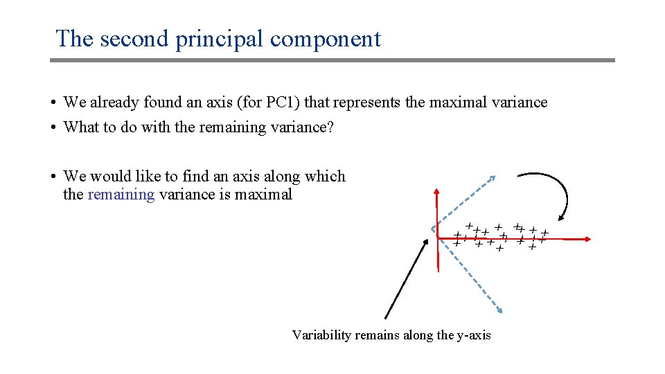
The second principal component • We already found an axis (for PC 1) that represents the maximal variance • What to do with the remaining variance? • We would like to find an axis along which the remaining variance is maximal xx xx xx x x xx Variability remains along the y-axis

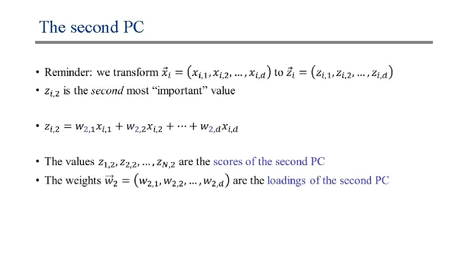
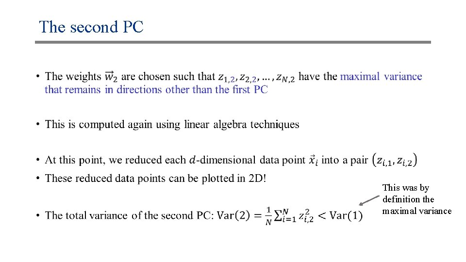
The second PC •

The second PC • This was by definition the maximal variance

An interactive visualization • http: //setosa. io/ev/principal-component-analysis/

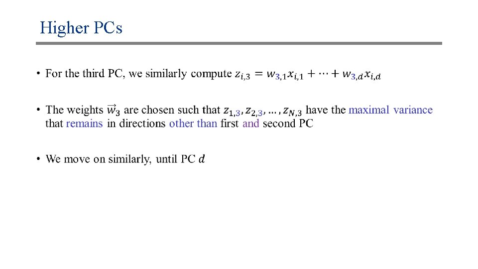
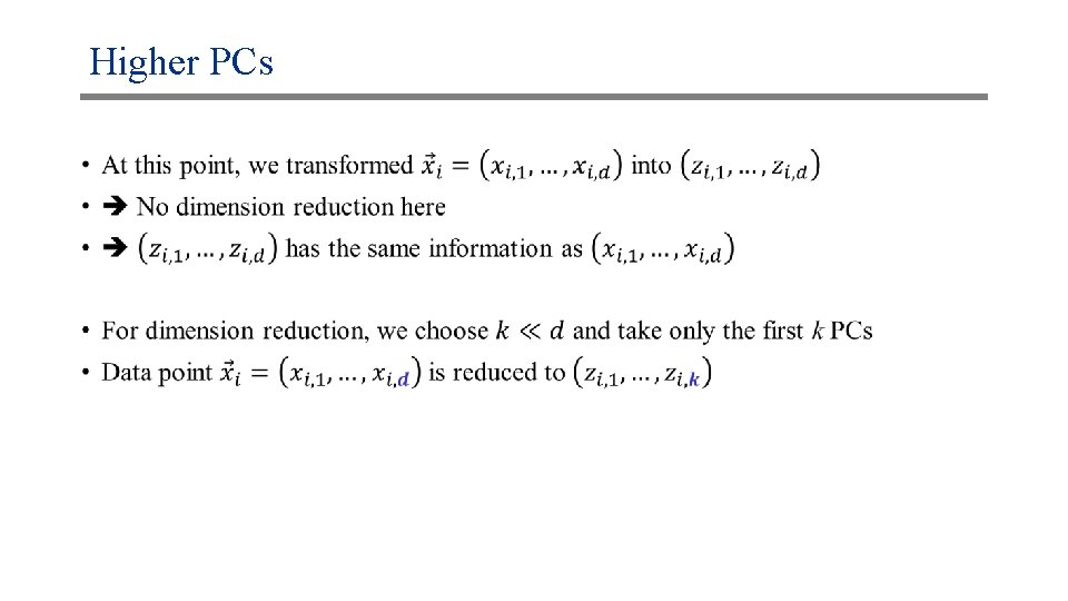
Higher PCs •

Higher PCs •

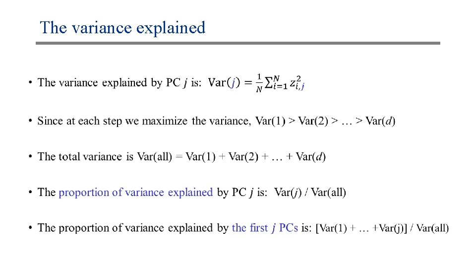
The variance explained •

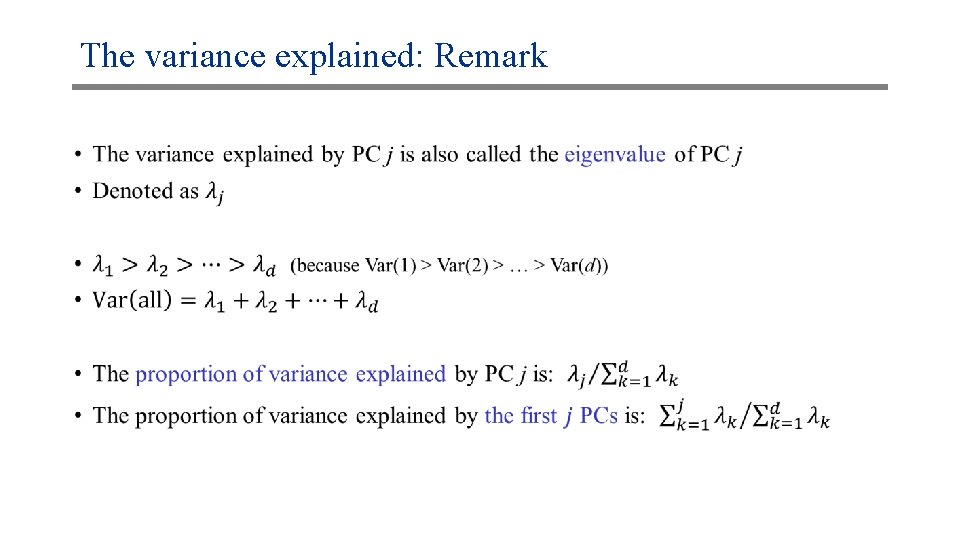
The variance explained: Remark •

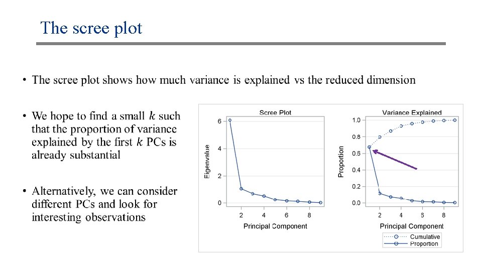
The scree plot •

PCA: Remarks • Sensitive to the scale of the data points (i. e. , different magnitudes of features) • Sensitive to imbalance between groups sizes, outliers • • Usages: Mostly for exploratory analysis Sometimes in regression/classification/clustering, to avoid the “curse of dimensionality” Can also be used as a means of data compression

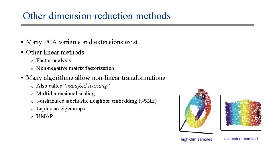
Other dimension reduction methods • Many PCA variants and extensions exist • Other linear methods: o o Factor analysis Non-negative matrix factorization • Many algorithms allow non-linear transformations o o o Also called “manifold learning” Multidimensional scaling t-distributed stochastic neighbor embedding (t-SNE) Laplacian eigenmaps UMAP