Advanced Topics in Artificial Intelligence for Intelligent Systems

Advanced Topics in Artificial Intelligence for Intelligent Systems (IN 5490): Classification Fall 2018 Enrique Garcia Ceja (enriqug@ifi. uio. no)

• Machine learning taxonomy. • Supervised learning. • Classification. • Imbalanced data. • Random over/under sampling. • SMOTE. • Cost‐sensitive classification. • Semi‐supervised learning. • Self‐learning. • Multi‐view learning. • Co‐Training. • Stacked generalization. • Data representations. • Multi‐user evaluation. • Baseline classifiers.

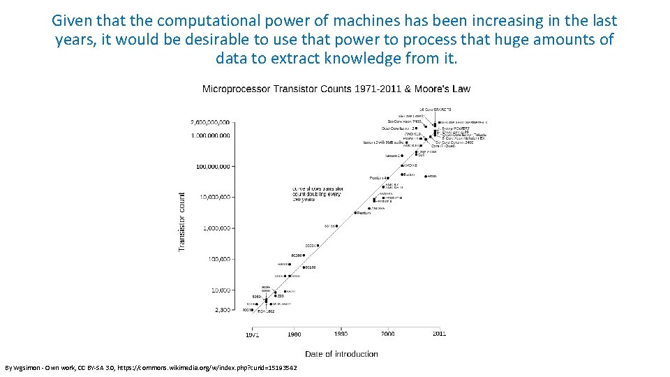
Big amounts of data With the advent of information technologies the amount of data that is generated everyday is growing at a fast pace. Trying to extract information and knowledge from that vast cumulus of data is a time consuming (if not impossible) task to do by hand.

Given that the computational power of machines has been increasing in the last years, it would be desirable to use that power to process that huge amounts of data to extract knowledge from it. By Wgsimon ‐ Own work, CC BY‐SA 3. 0, https: //commons. wikimedia. org/w/index. php? curid=15193542

Machine learning can be thought of (but not limited to), as a set of computational algorithms that automatically find interesting patterns and relationships from data. “The basic principle of machine learning is the automatic modeling of underlying processes that have generated the collected data. ” (I. Kononenko and M. Kukar, 2007).

Learning • (I. Kononenko and M. Kukar. , 2007) defined learning as “any modification of the system that improves its performance in some problem solving task. ” • The result of learning is knowledge that the system can use to solve new problems. An algorithm infers the properties of a given set of data and that information allows it to make predictions about other data that it might see in the future. • This is possible because almost all nonrandom data contains patterns which allows a machine to generalize (T. Segaran, 2007).

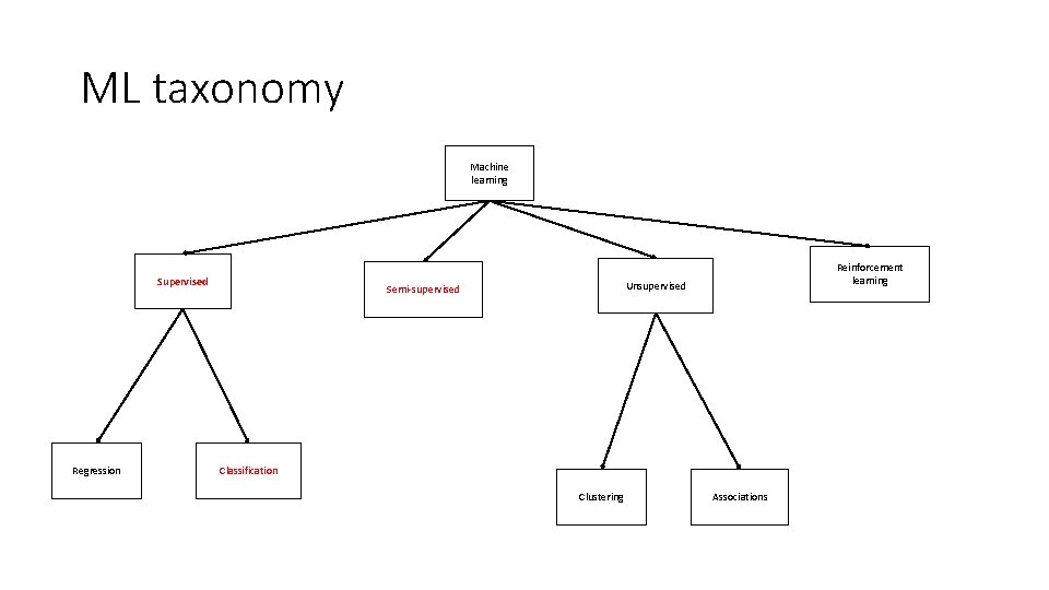
ML taxonomy Machine learning Supervised Regression Reinforcement learning Unsupervised Semi‐supervised Classification Clustering Associations

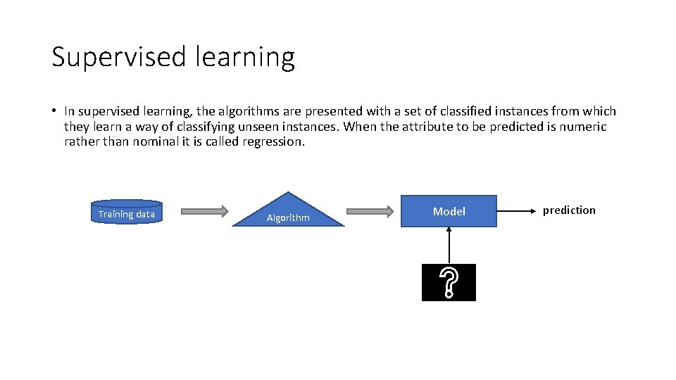
Supervised learning • In supervised learning, the algorithms are presented with a set of classified instances from which they learn a way of classifying unseen instances. When the attribute to be predicted is numeric rather than nominal it is called regression. Training data Algorithm Model prediction

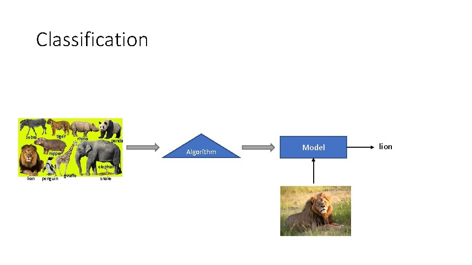
Classification zebra tiger rhino panda Algorithm hippo elephant lion penguin giraffe snake Model lion

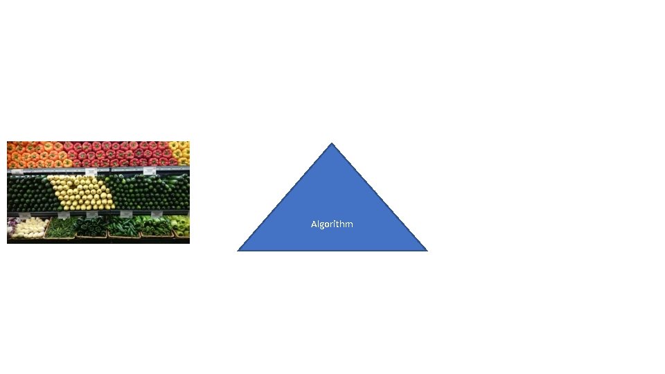
Remember: garbage in, garbage out Algorithm

Algorithm

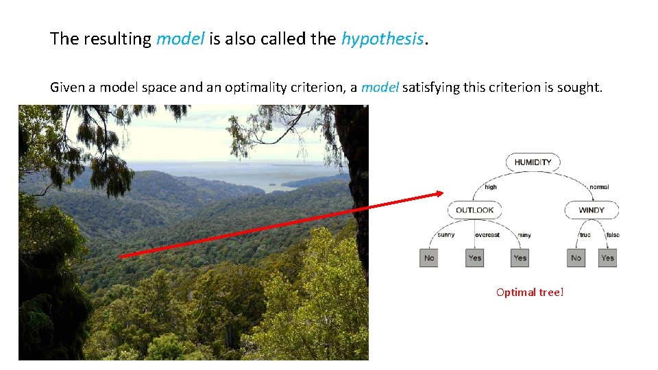
The resulting model is also called the hypothesis. Given a model space and an optimality criterion, a model satisfying this criterion is sought. Optimal tree!

Some criteria: • Maximizing the prediction accuracy • Minimizing the hypothesis’ size • Maximizing the hypothesis fitness to the input data • Maximizing the hypothesis interpretability • Minimizing the time complexity of prediction

Imbalanced data • Random over/under sampling • SMOTE • Cost sensitive classification

You trained a model to predict cancer from image data using a state of the art Hierarchical siamese CNN with dynamic kernel activations…

Your model has an accuracy of 99. 9%

But… WTH!?

By looking at the confusion matrix you realize that the model does not detect any of the positive examples.

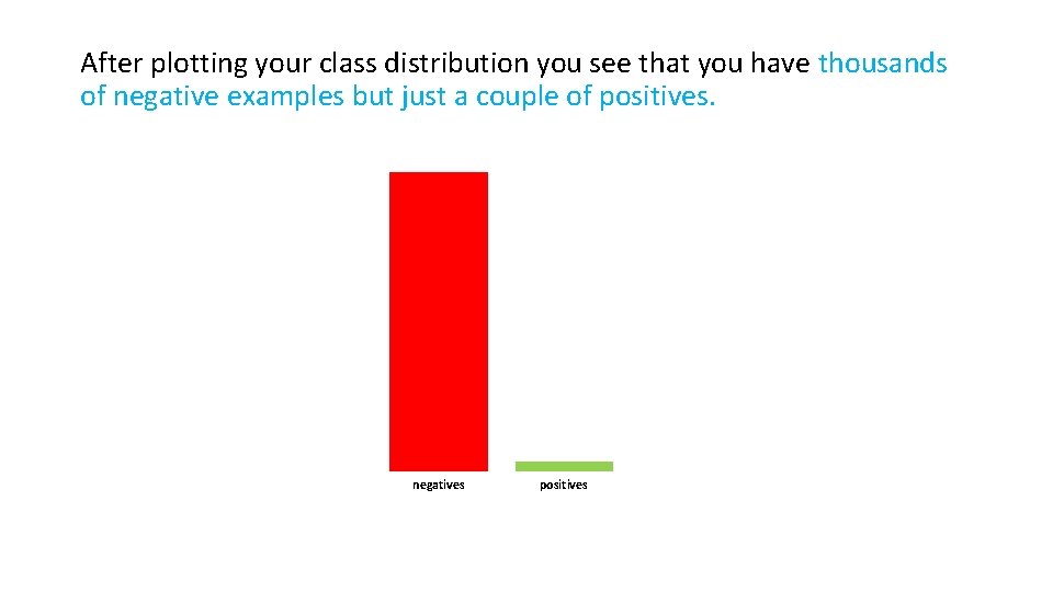
After plotting your class distribution you see that you have thousands of negative examples but just a couple of positives. negatives positives

Classifiers try to reduce the overall error so they can be biased towards the majority class. # Negatives = 998 # Positives = 2 By always predicting a negative class the accuracy will be 99. 8% !!

Your dataset is imbalanced. Now what? ?

What can you do? • Collect more data (difficult in many domains) • Delete data from the majority class • Create synthetic data • Adapt your learning algorithm (cost sensitive classification)

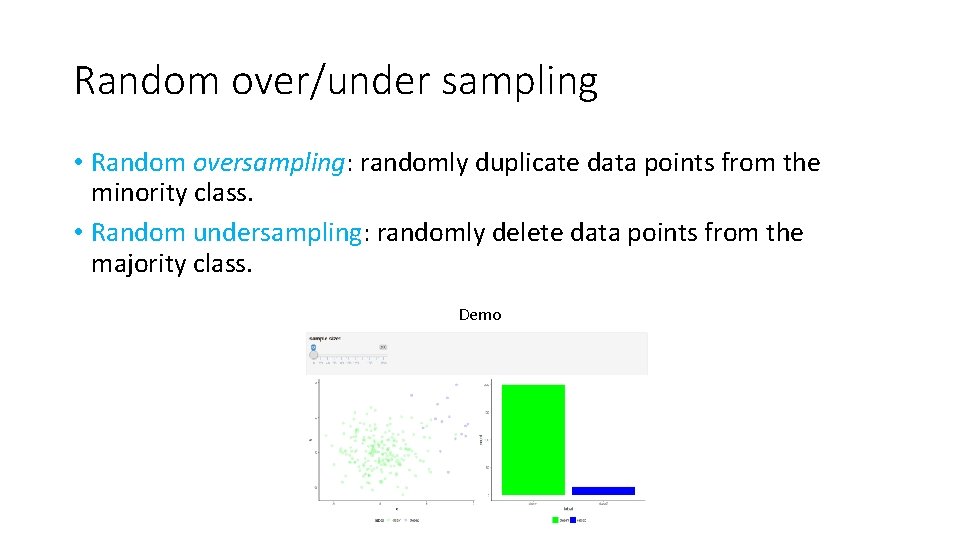
Random over/under sampling • Random oversampling: randomly duplicate data points from the minority class. • Random undersampling: randomly delete data points from the majority class. Demo

Problems with these approaches: • Loss of information (in the case of under sampling) • Overfitting and fixed boundaries (over sampling)

SMOTE • Synthetic Minority Over‐sampling Technique (Chawla). • Creates new data points from the minority class. • Operates in the feature space.

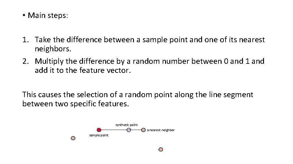
• Main steps: 1. Take the difference between a sample point and one of its nearest neighbors. 2. Multiply the difference by a random number between 0 and 1 and add it to the feature vector. This causes the selection of a random point along the line segment between two specific features. synthetic point a nearest neighbor sample point

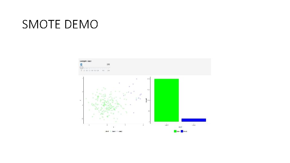
SMOTE DEMO

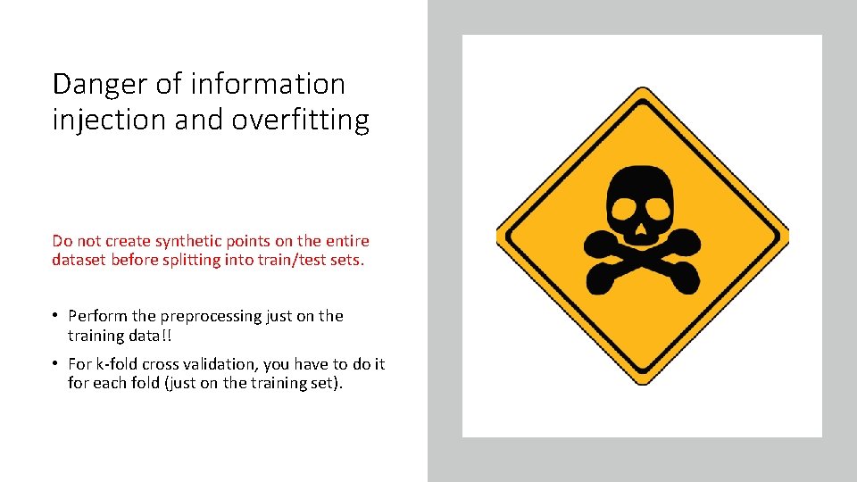
Danger of information injection and overfitting Do not create synthetic points on the entire dataset before splitting into train/test sets. • Perform the preprocessing just on the training data!! • For k‐fold cross validation, you have to do it for each fold (just on the training set).

For images: • Augment training data by applying image transformations: rotate, scale, shift, etc. • Keras provides functionalities for data augmentation: https: //blog. keras. io/building‐powerful‐image‐classification‐models‐ using‐very‐little‐data. html

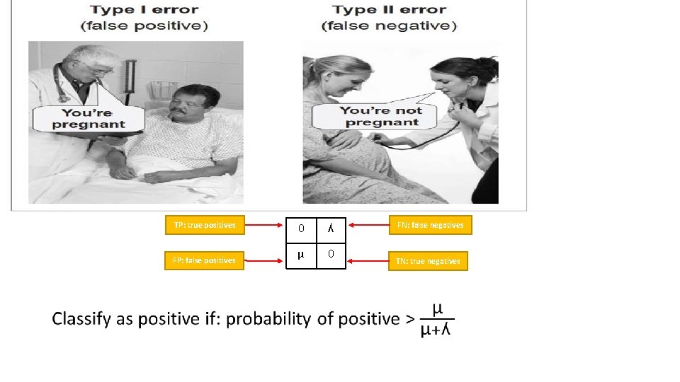
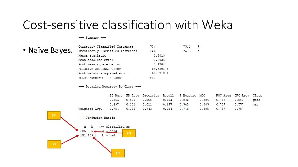
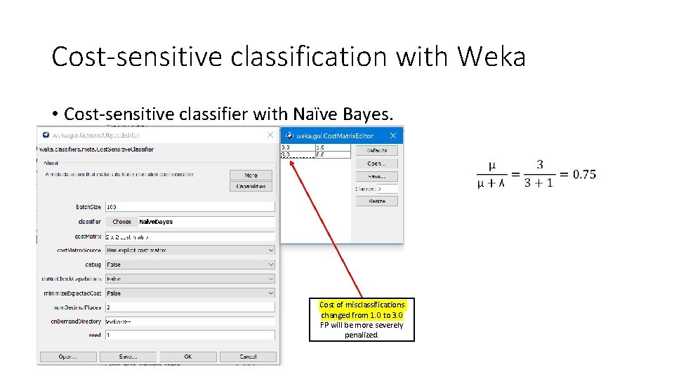
Cost-sensitive classification • TP: true positives FP: false positives 0 ʎ µ 0 FN: false negatives TN: true negatives

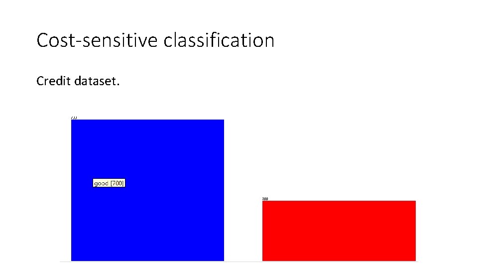
Cost-sensitive classification Credit dataset.

Cost-sensitive classification with Weka • Naïve Bayes. TP FN FP TN

Cost-sensitive classification with Weka • Cost‐sensitive classifier with Naïve Bayes. Cost of misclassifications changed from 1. 0 to 3. 0 FP will be more severely penalized.

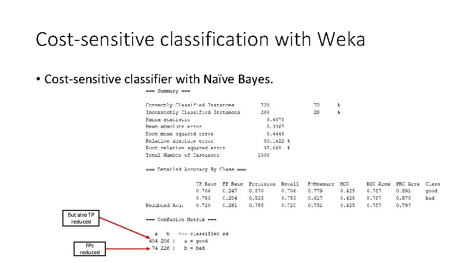
Cost-sensitive classification with Weka • Cost‐sensitive classifier with Naïve Bayes. But also TP reduced FPs reduced

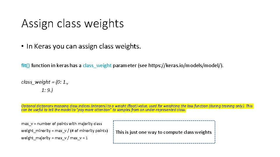
Assign class weights • In Keras you can assign class weights. fit() function in keras has a class_weight parameter (see https: //keras. io/models/model/). class_weight = {0: 1. , 1: 9. } Optional dictionary mapping class indices (integers) to a weight (float) value, used for weighting the loss function (during training only). This can be useful to tell the model to "pay more attention" to samples from an under-represented class. max_v = number of points with majority class weight_minority = max_v / (# of minority points) weight_majority = max_v / max_v = 1 This is just one way to compute class weights

Tools • Python imbalanced‐learn library: https: //github. com/scikit‐learn‐ contrib/imbalanced‐learn • Weka also has oversampling methods and a cost sensitive meta classifier: https: //weka. wikispaces. com/Cost. Sensitive. Classifier

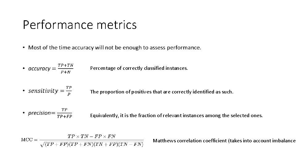
Performance metrics • Percentage of correctly classified instances. The proportion of positives that are correctly identified as such. Equivalently, it is the fraction of relevant instances among the selected ones. Matthews correlation coefficient (takes into account imbalance)

Supporting materials: imbalanced data • Chawla, N. V. , Bowyer, K. W. , Hall, L. O. , & Kegelmeyer, W. P. (2002). SMOTE: synthetic minority over‐ sampling technique. Journal of artificial intelligence research, 16, 321‐ 357. • Kotsiantis, S. , Kanellopoulos, D. , & Pintelas, P. (2006). Handling imbalanced datasets: A review. GESTS International Transactions on Computer Science and Engineering, 30(1), 25‐ 36. • Python imbalanced‐learn library: https: //github. com/scikit‐learn‐contrib/imbalanced‐learn • Weka also has oversampling methods and a cost sensitive meta classifier: https: //weka. wikispaces. com/Cost. Sensitive. Classifier • Cost‐sensitive classification video: https: //www. youtube. com/watch? v=l 9 mu. Pld. OG 30 • Performance metrics: https: //en. wikipedia. org/wiki/Sensitivity_and_specificity

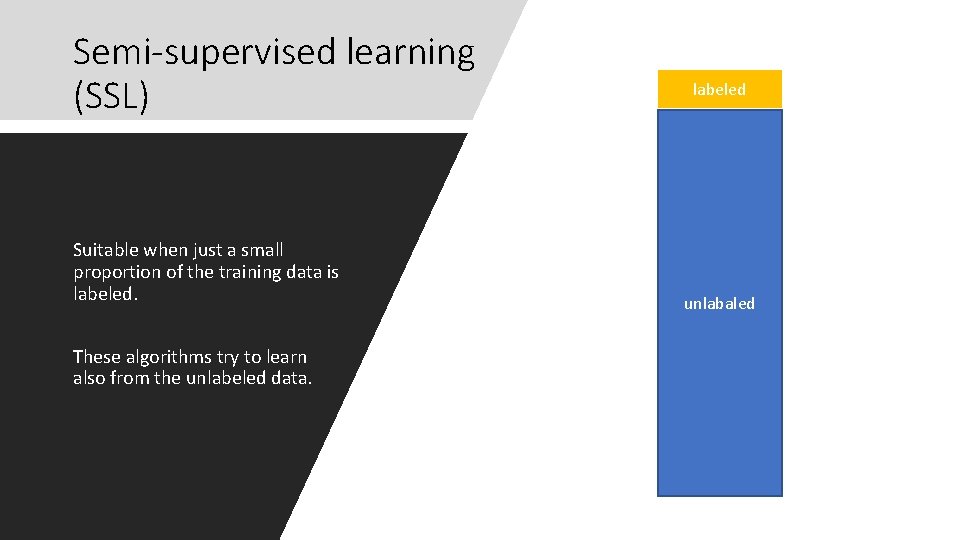
Semi-supervised learning (SSL) Suitable when just a small proportion of the training data is labeled. These algorithms try to learn also from the unlabeled data. labeled unlabaled

Semi-supervised learning (SSL) Suitable for datasets with: • Small amounts of labeled data • Large amounts of unlabeled data (labeling requires effort) • High certainty in labels

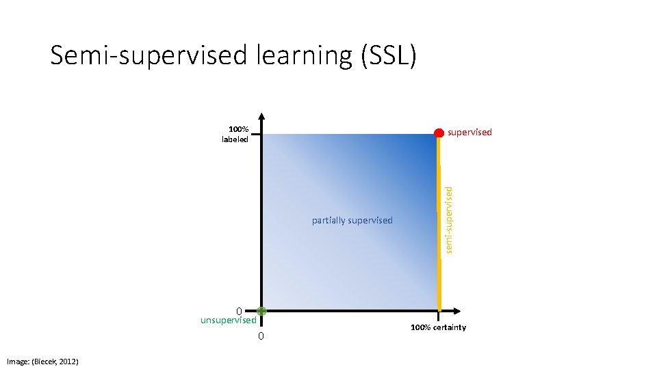
Semi-supervised learning (SSL) 100% labeled partially supervised semi‐supervised 0 unsupervised 0 Image: (Biecek, 2012) 100% certainty

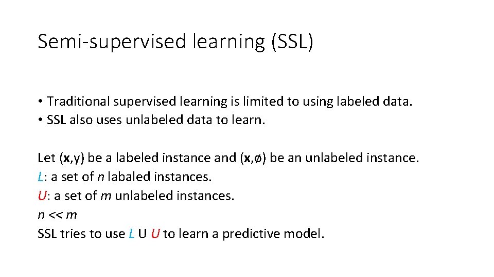
Semi-supervised learning (SSL) • Traditional supervised learning is limited to using labeled data. • SSL also uses unlabeled data to learn. Let (x, y) be a labeled instance and (x, ø) be an unlabeled instance. L: a set of n labaled instances. U: a set of m unlabeled instances. n << m SSL tries to use L U U to learn a predictive model.

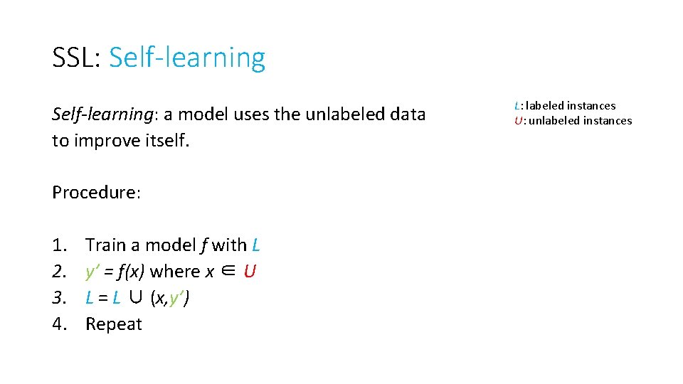
SSL: Self-learning: a model uses the unlabeled data to improve itself. Procedure: 1. 2. 3. 4. Train a model f with L y’ = f(x) where x ∈ U L = L ∪ (x, y’) Repeat L: labeled instances U: unlabeled instances

Self-learning ‘improvements’ • Just add instances with the most confident predictions. • Perform the procedure with batches of instances instead of one instance at a time. • Re‐assess previous predictions.

SSL is not always guaranteed to work! Performance may also degrade due to noisy instances. Remember: garbage in, garbage out! 40

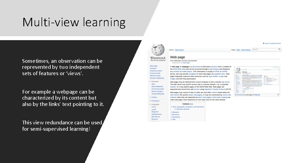
Multi-view learning Sometimes, an observation can be represented by two independent sets of features or ‘views’. For example a webpage can be characterized by its content but also by the links’ text pointing to it. This view redundance can be used for semi‐supervised learning!

Multi-view learning • Conventional algorithms ‘concatenate’ all views. • This approach might cause overfitting with small training sets. • Not physically meaningful since each view has specific statistical properties.

Multi-view learning Multi‐view learning takes advantage of all views to jointly optimize and exploit the redundant views of the same input data to improve performance.

Multi-view learning Co‐Training (Blum, A. , & Mitchell, T. ) is a type of semi‐supervised algorithm. Two classifiers work together to enlarge the training set L and increase performance.

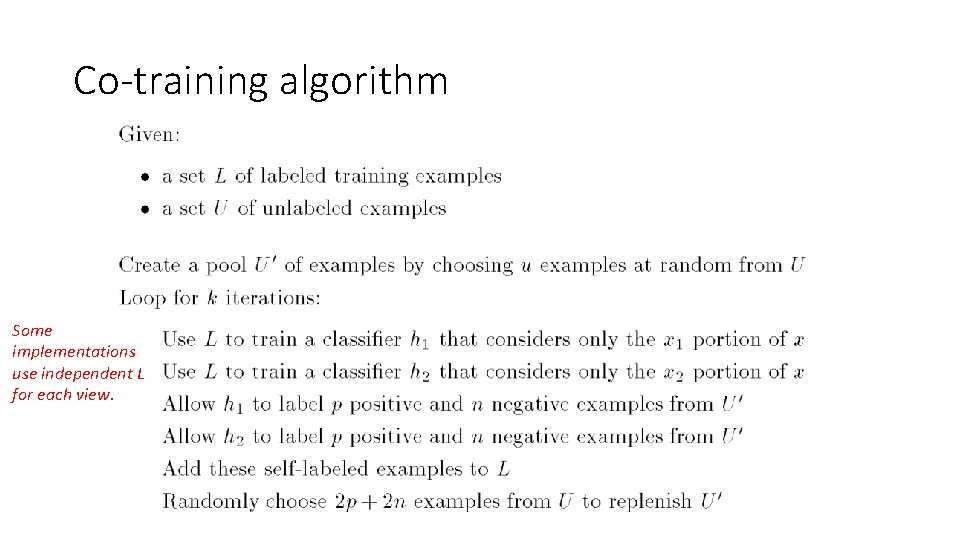
Co-training algorithm Some implementations use independent L for each view.

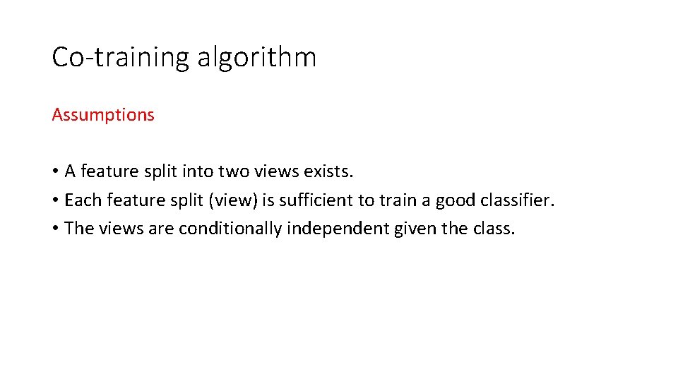
Co-training algorithm Assumptions • A feature split into two views exists. • Each feature split (view) is sufficient to train a good classifier. • The views are conditionally independent given the class.

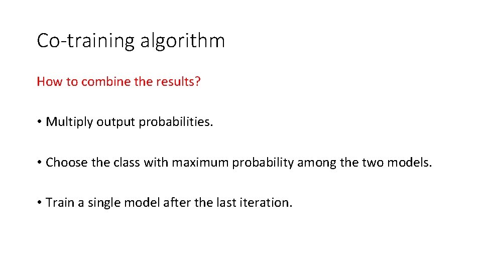
Co-training algorithm How to combine the results? • Multiply output probabilities. • Choose the class with maximum probability among the two models. • Train a single model after the last iteration.

Tri-training Tri‐training (Zhou and Li) • Use three learners. If two agree, the data is used to teach the third learner.

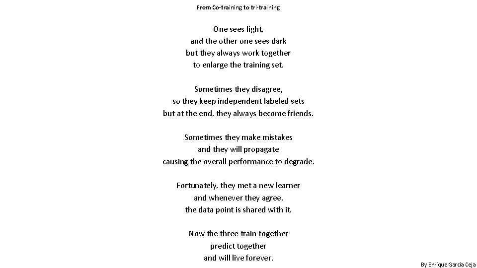
From Co-training to tri-training One sees light, and the other one sees dark but they always work together to enlarge the training set. Sometimes they disagree, so they keep independent labeled sets but at the end, they always become friends. Sometimes they make mistakes and they will propagate causing the overall performance to degrade. Fortunately, they met a new learner and whenever they agree, the data point is shared with it. Now the three train together predict together and will live forever. By Enrique Garcia Ceja

Supporting materials: SSL, multi-view learning and co-training. • Blum, A. , & Mitchell, T. (1998, July). Combining labeled and unlabeled data with co‐training. In Proceedings of the eleventh annual conference on Computational learning theory (pp. 92‐ 100). ACM. • Zhou, Z. H. , & Li, M. (2005). Tri‐training: Exploiting unlabeled data using three classifiers. IEEE Transactions on knowledge and Data Engineering, 17(11), 1529‐ 1541. • Chapelle, O. , Scholkopf, B. , & Zien, A. (2009). Semi‐supervised learning (chapelle, o. et al. , eds. ; 2006)[book reviews]. IEEE Transactions on Neural Networks, 20(3), 542‐ 542.

Stacked Generalization

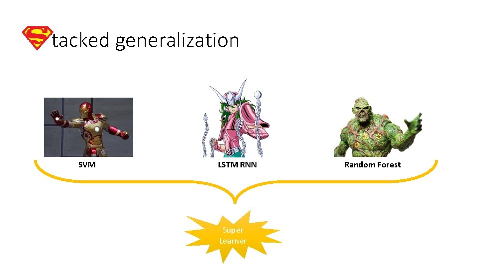
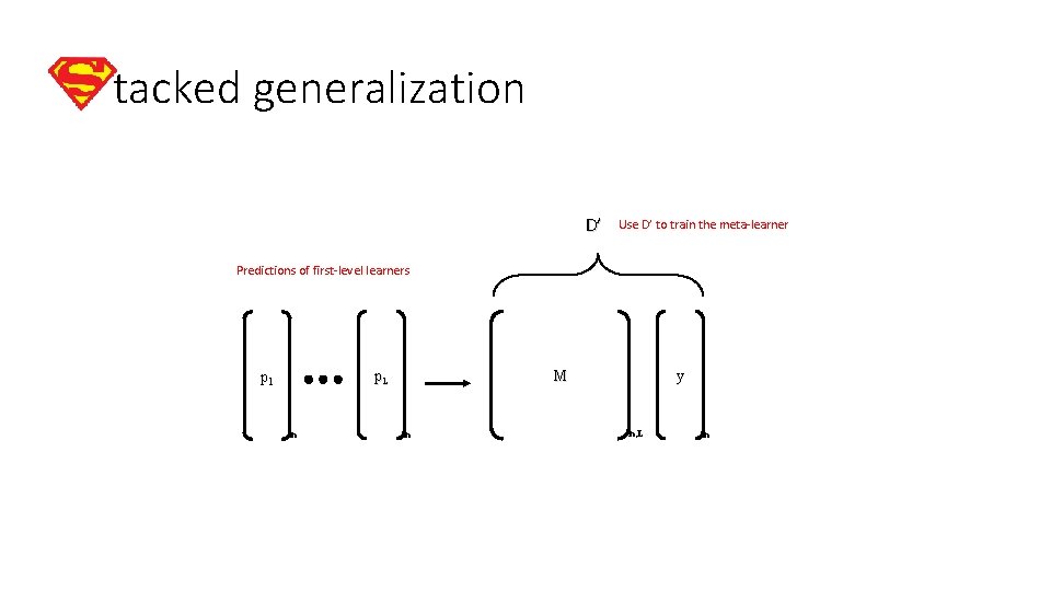
tacked generalization • Proposed by (Wolpert, 1992). • Combines a set of powerful learners by stacking their outputs. • Many of the Kaggle’s winning solutions use some type of stacking.

tacked generalization SVM LSTM RNN Super Learner Random Forest

tacked generalization • First, train a set of first-level learners. • Use the outputs of the first-level learners to train a meta-learner.

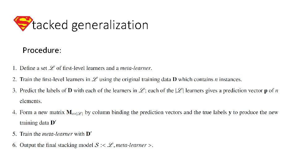
tacked generalization Procedure:

tacked generalization D’ Use D’ to train the meta‐learner Predictions of first‐level learners M p. L p 1 n n y n, L n

tacked generalization • Steps 2 and 3 can lead to overfitting. • To avoid this, use k‐fold cross validation within these steps. • After D’ has been generated, retrain all first‐level learners with all data from D.

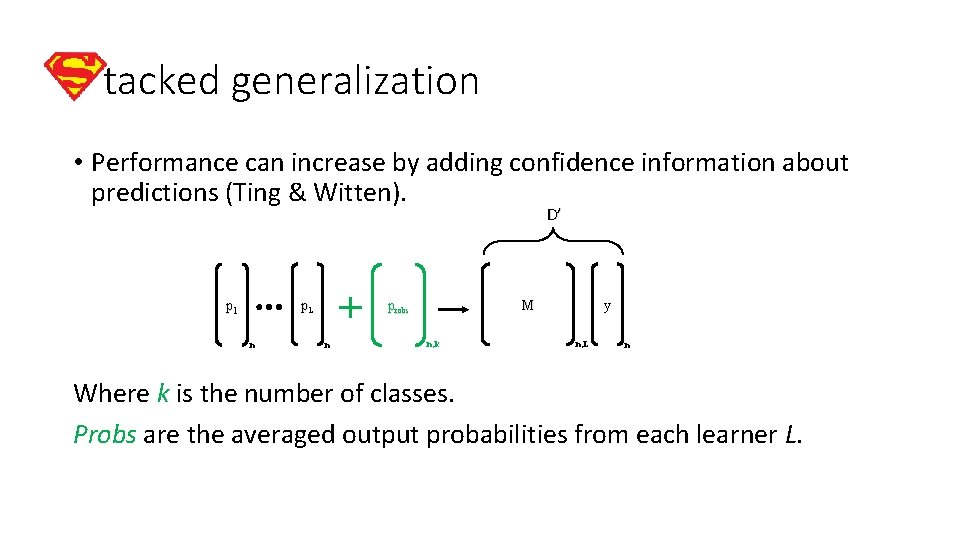
tacked generalization • Performance can increase by adding confidence information about predictions (Ting & Witten). D’ p. L p 1 n M probs n n, k y n, L n Where k is the number of classes. Probs are the averaged output probabilities from each learner L.

Supporting materials: stacked generalization • Zhou, Z. H. (2012). Ensemble methods: foundations and algorithms. Chapman and Hall/CRC. • Wolpert, D. H. (1992). Stacked generalization. Neural networks, 5(2), 241‐ 259.

Data representations

• Selecting a data representation is crucial. • Invest time thinking about the possibilities. • Each representation provides a different perspective/view (information). • Predictive models will depend on the type of representation.

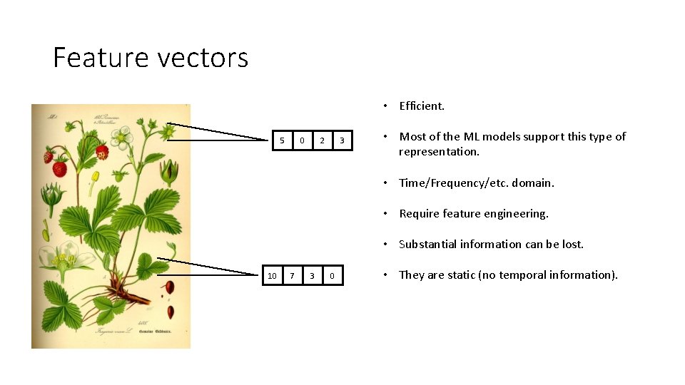
Feature vectors • Efficient. 5 0 2 3 • Most of the ML models support this type of representation. • Time/Frequency/etc. domain. • Require feature engineering. • Substantial information can be lost. 10 7 3 0 • They are static (no temporal information).

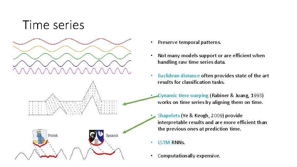
Time series • Preserve temporal patterns. • Not many models support or are efficient when handling raw time series data. • Euclidean distance often provides state of the art results for classification tasks. • Dynamic time warping (Rabiner & Juang, 1993) works on time series by aligning them on time. • Shapelets (Ye & Keogh, 2009) provide interpretable results and are more efficient than the previous ones at prediction time. • LSTM RNNs. • Computationally expensive.

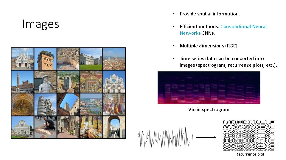
Images • Provide spatial information. • Efficient methods: Convolutional Neural Networks CNNs. • Multiple dimensions (RGB). • Time series data can be converted into images (spectrogram, recurrence plots, etc. ). Violin spectrogram Recurrence plot

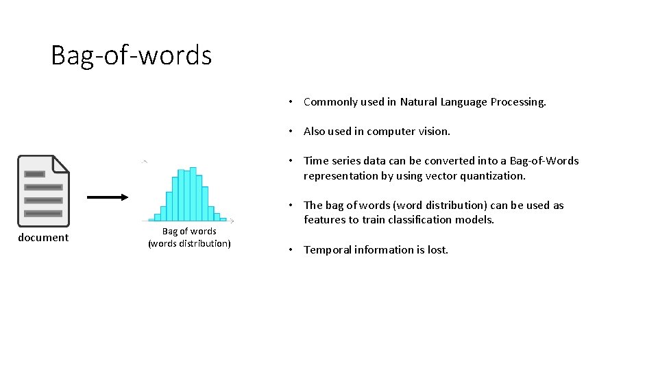
Bag-of-words • Commonly used in Natural Language Processing. • Also used in computer vision. • Time series data can be converted into a Bag‐of‐Words representation by using vector quantization. document Bag of words (words distribution) • The bag of words (word distribution) can be used as features to train classification models. • Temporal information is lost.

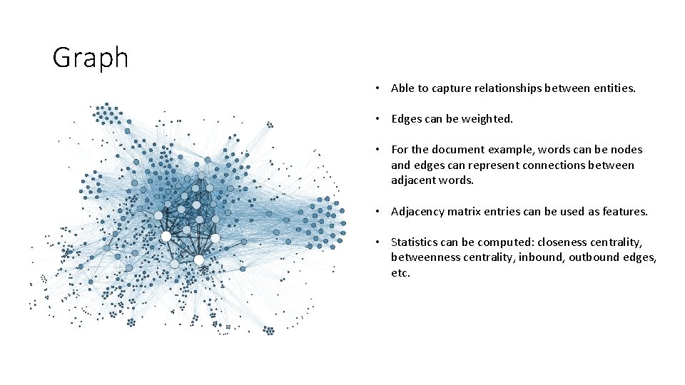
Graph • Able to capture relationships between entities. • Edges can be weighted. • For the document example, words can be nodes and edges can represent connections between adjacent words. • Adjacency matrix entries can be used as features. • Statistics can be computed: closeness centrality, betweenness centrality, inbound, outbound edges, etc.

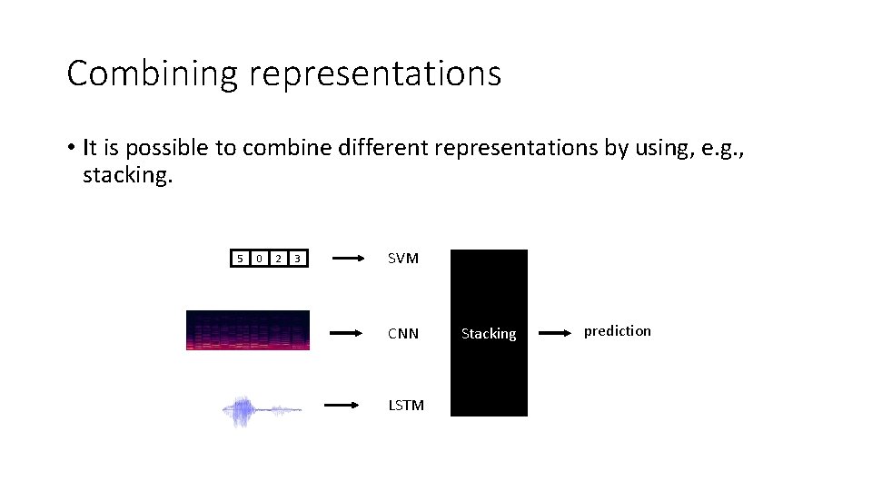
Combining representations • It is possible to combine different representations by using, e. g. , stacking. 5 0 2 3 SVM CNN LSTM Stacking prediction

Multi-user evaluation Evaluate classification models in multi‐user settings.

Behavior differences • Users are unique. • Possess different characteristics and behaviors. • Attributes: age, gender, height, etc.

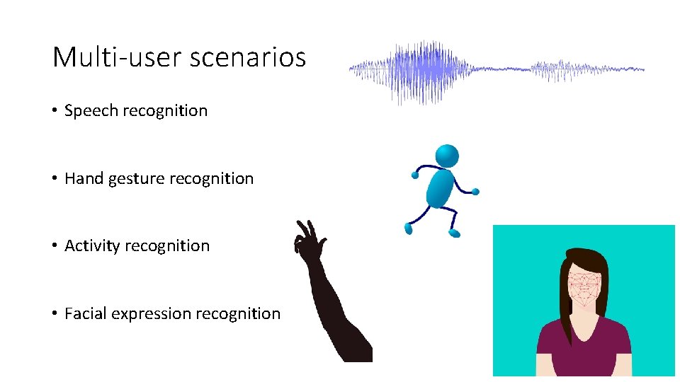
Multi-user scenarios • Speech recognition • Hand gesture recognition • Activity recognition • Facial expression recognition

Evaluation types • Mixed models • General models (user‐independent models) • Personal models (user‐dependent)

Mixed models • Do not make distinction between users. • Training/testing sets generated independently of users. • Some data points of the same user can be in both training and testing sets. • Performance results may not be representative of how the system will perform in real life. Using a mixed model in multi‐user scenarios is not a good idea to assess performance.

Personal models (user-dependent) • Are trained with data just from the same user. • In general, their performance is the best. • They require more data for each particular user. • Prone to overfitting.

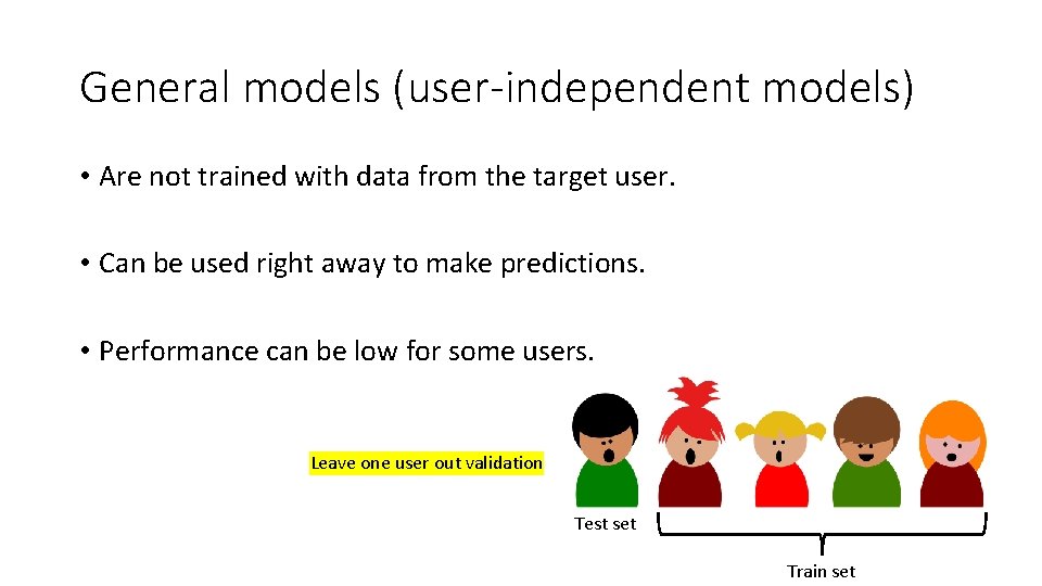
General models (user-independent models) • Are not trained with data from the target user. • Can be used right away to make predictions. • Performance can be low for some users. Leave one user out validation Test set Train set

Supporting materials: Multi-user evaluation • Lockhart, J. W. , & Weiss, G. M. (2014, April). The benefits of personalized smartphone‐based activity recognition models. In Proceedings of the 2014 SIAM international conference on data mining (pp. 614‐ 622). Society for Industrial and Applied Mathematics. • Rokni, S. A. , Nourollahi, M. , & Ghasemzadeh, H. (2018). Personalized Human Activity Recognition Using Convolutional Neural Networks. ar. Xiv preprint ar. Xiv: 1801. 08252.

Baseline classifiers • Machine learning is not the answer to every problem. • You can solve many problems with simple heuristics. • Assess whether or not machine learning has a benefit.

Baseline classifiers • Predict the most frequent class. • Predict according to class distributions. • Predict uniformly at random. • Predict the average value. • Predict next observations as the value of the previous one.

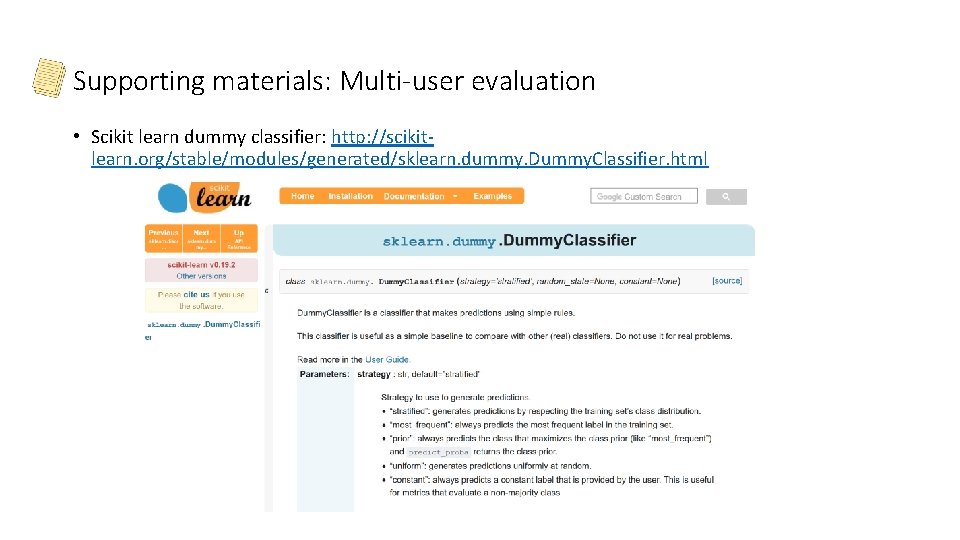
Supporting materials: Multi-user evaluation • Scikit learn dummy classifier: http: //scikit‐ learn. org/stable/modules/generated/sklearn. dummy. Dummy. Classifier. html

QUESTIONS? • Machine learning taxonomy. • Supervised learning. • Classification. • Imbalanced data. • Random over/under sampling. • SMOTE. • Cost‐sensitive classification. • Semi‐supervised learning. • Self‐learning. • Multi‐view learning. • Co‐Training. • Stacked generalization. • Data representations. • Multi‐user evaluation. • Baseline classifiers

References • I. Kononenko and M. Kukar. Machine Learning and Data Mining. Horwood Publishing, 2007. • T. Segaran. Programming Collective Intelligence: Building Smart Web 2. 0 Applications. Oreilly Series. O'Reilly Media, 2007. • Jenkins, A. L. , Singer, J. , Conner, B. T. , Calhoun, S. , & Diamond, G. (2014). Risk for Suicidal Ideation and Attempt among a Primary Care Sample of Adolescents Engaging in Nonsuicidal Self‐Injury. Suicide and life-threatening behavior, 44(6), 616‐ 628. • Dinsha, D. and Manikandaprabu, N. , 2014. Breast tumor segmentation and classification using SVM and Bayesian from thermogram images. Unique Journal of Engineering and Advanced Sciences, 2(2), pp. 147‐ 151. • Chawla, N. V. , Bowyer, K. W. , Hall, L. O. , & Kegelmeyer, W. P. (2002). SMOTE: synthetic minority over‐sampling technique. Journal of artificial intelligence research, 16, 321‐ 357. • law Biecek, P. , Szczurek, E. , Vingron, M. , & Tiuryn, J. The R Package bgmm: Mixture Modeling with Uncertain Knowledge. • Blum, A. , & Mitchell, T. (1998, July). Combining labeled and unlabeled data with co‐training. In Proceedings of the eleventh annual conference on Computational learning theory (pp. 92‐ 100). ACM. • Zhou, Z. H. , & Li, M. (2005). Tri‐training: Exploiting unlabeled data using three classifiers. IEEE Transactions on knowledge and Data Engineering, 17(11), 1529‐ 1541. • Wolpert, D. H. (1992). Stacked generalization. Neural networks, 5(2), 241‐ 259. • Ting, K. M. , & Witten, I. H. (1999). Issues in stacked generalization. Journal of artificial intelligence research, 10, 271‐ 289. • Rabiner, L. R. , & Juang, B. H. (1993). Fundamentals of speech recognition (Vol. 14). Englewood Cliffs: PTR Prentice Hall. • Ye, L. , & Keogh, E. (2009, June). Time series shapelets: a new primitive for data mining. In Proceedings of the 15 th ACM SIGKDD international conference on Knowledge discovery and data mining (pp. 947‐ 956). ACM.