Advanced Statistics I Xiayu Stacy Huang Bioinformatics Shared

Advanced Statistics I Xiayu (Stacy) Huang Bioinformatics Shared Resource Sanford | Burnham Medical Research Institute

Outline § Summary of Previous Talk § Descriptive & inferential statistics § T test § Common statistical tests and Applications (Continue) § One-way ANOVA § Post hoc/multiple comparison tests § One-way ANOVA power analysis § Common data transformation methods

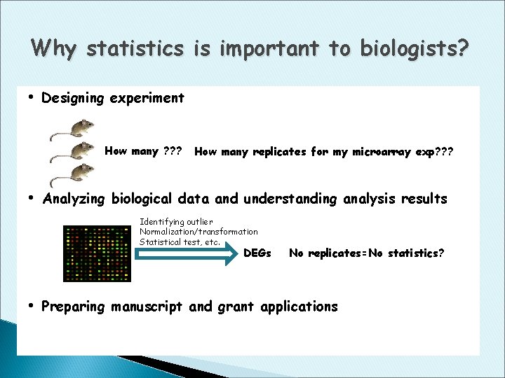
Why statistics is important to biologists? • Designing experiment How many ? ? ? How many replicates for my microarray exp? ? ? • Analyzing biological data and understanding analysis results Identifying outlier Normalization/transformation Statistical test, etc. DEGs No replicates=No statistics? • Preparing manuscript and grant applications

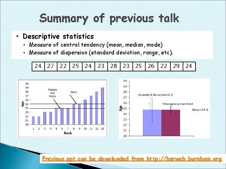
Summary of previous talk • Descriptive statistics • Measure of central tendency (mean, median, mode) • Measure of dispersion (standard deviation, range, etc). 24 27 22 25 24 23 28 23 25 26 22 29 24 Previous ppt can be downloaded from http: //bsrweb. burnham. org

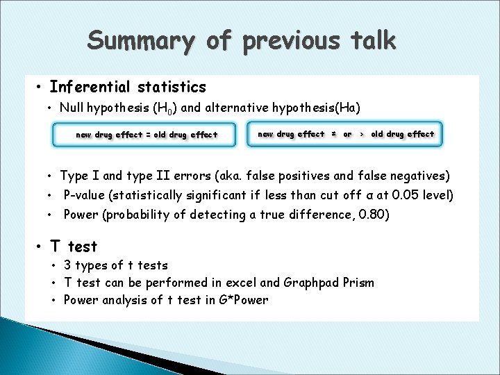
Summary of previous talk • Inferential statistics • Null hypothesis (H 0) and alternative hypothesis(Ha) new drug effect = old drug effect new drug effect ≠ or > old drug effect • Type I and type II errors (aka. false positives and false negatives) • P-value (statistically significant if less than cut off α at 0. 05 level) • Power (probability of detecting a true difference, 0. 80) • T test • 3 types of t tests • T test can be performed in excel and Graphpad Prism • Power analysis of t test in G*Power

Analysis of variance (ANOVA) Overview ◦ History of ANOVA Ronald Fisher proposed ANOVA in 1918 His first application of ANOVA was published in 1921 ◦ What does ANOVA do? Comparing the means of 3 or more populations without knowing the exact difference between population means ◦ Types of ANOVA One-way and multi-way ANOVA (# of factors of interest) Repeated measures ANOVA (repeated measurements on the same subject) MANOVA (# of different measurements)

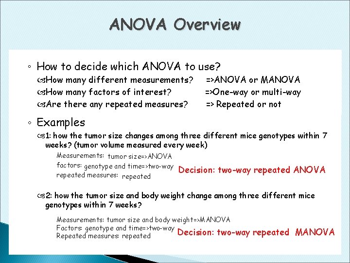
ANOVA Overview ◦ How to decide which ANOVA to use? How many different measurements? How many factors of interest? Are there any repeated measures? =>ANOVA or MANOVA =>One-way or multi-way => Repeated or not ◦ Examples 1: how the tumor size changes among three different mice genotypes within 7 weeks? (tumor volume measured every week) Measurements: tumor size=>ANOVA factors: genotype and time=>two-way repeated measures: repeated Decision: two-way repeated ANOVA 2: how the tumor size and body weight change among three different mice genotypes within 7 weeks? Measurements: tumor size and body weight=>MANOVA Factors: genotype and time=>two-way Decision: two-way Repeated measures: repeated MANOVA

ANOVA application in biology One-way ANOVA Two-way repeated ANOVA Two-way ANOVA One-way MANOVA

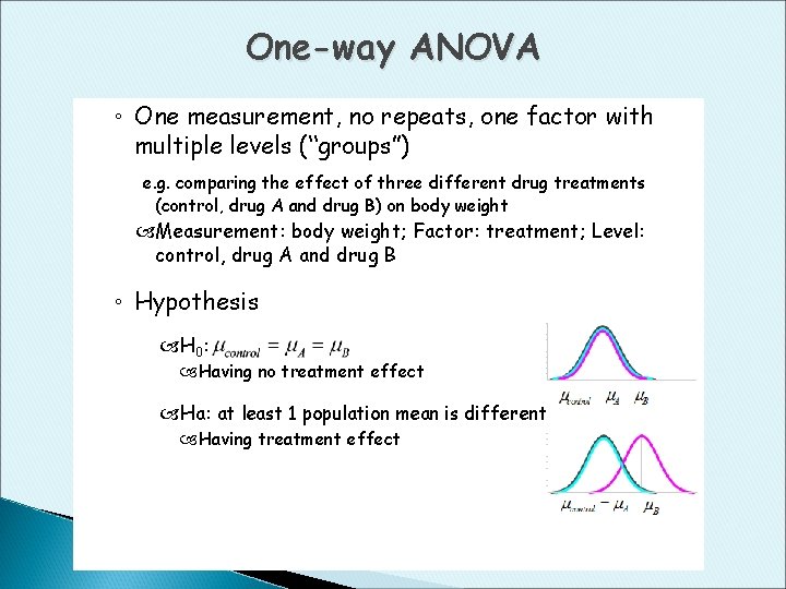
One-way ANOVA ◦ One measurement, no repeats, one factor with multiple levels (“groups”) e. g. comparing the effect of three different drug treatments (control, drug A and drug B) on body weight Measurement: body weight; Factor: treatment; Level: control, drug A and drug B ◦ Hypothesis H 0: Having no treatment effect Ha: at least 1 population mean is different Having treatment effect

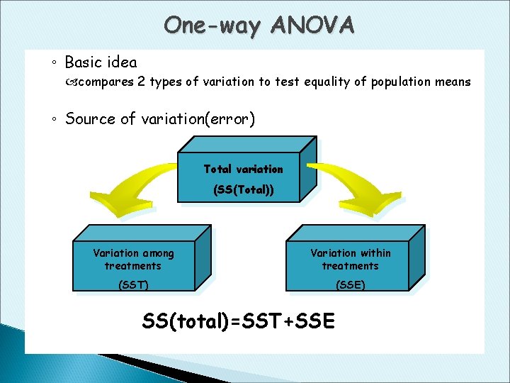
One-way ANOVA ◦ Basic idea compares 2 types of variation to test equality of population means ◦ Source of variation(error) Total variation (SS(Total)) Variation among treatments Variation within treatments (SST) (SSE) SS(total)=SST+SSE

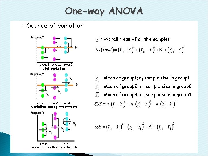
One-way ANOVA ◦ Source of variation : overall mean of all the samples group 1 group 2 group 3 total variation : Mean of group 1; n 1: sample size in group 1 : Mean of group 2; n 2: sample size in group 2 : Mean of group 3; n 3: sample size in group 3 group 1 group 2 group 3 variation among treatments group 1 group 2 group 3 variation within treatments

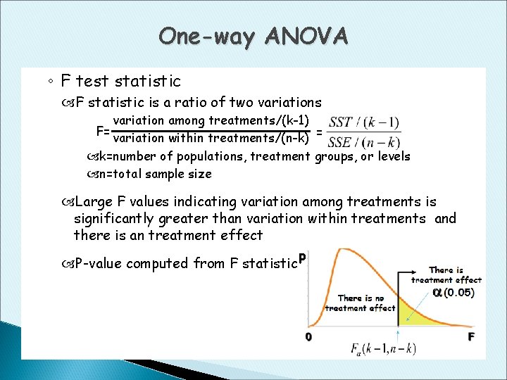
One-way ANOVA ◦ F test statistic F statistic is a ratio of two variations variation among treatments/(k-1) F= variation within treatments/(n-k) = k=number of populations, treatment groups, or levels n=total sample size Large F values indicating variation among treatments is significantly greater than variation within treatments and there is an treatment effect P-value computed from F statistic p

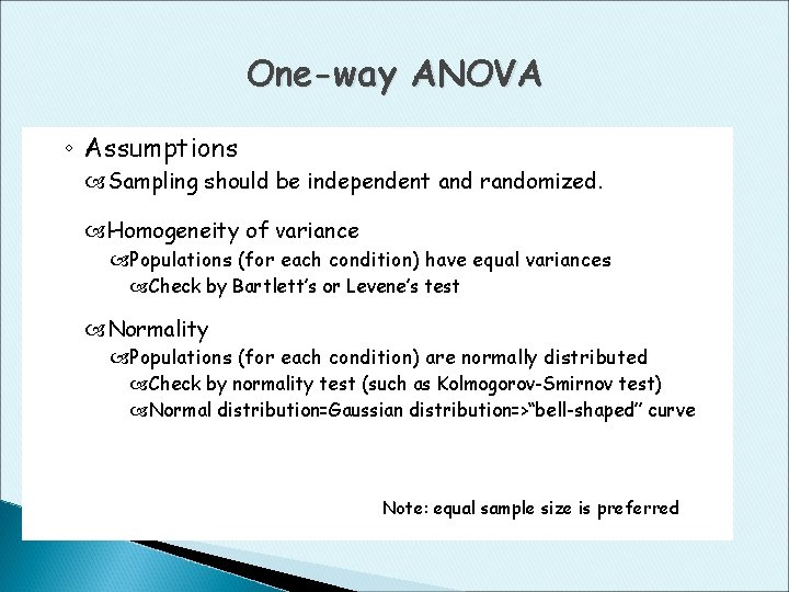
One-way ANOVA ◦ Assumptions Sampling should be independent and randomized. Homogeneity of variance Populations (for each condition) have equal variances Check by Bartlett’s or Levene’s test Normality Populations (for each condition) are normally distributed Check by normality test (such as Kolmogorov-Smirnov test) Normal distribution=Gaussian distribution=>“bell-shaped” curve Note: equal sample size is preferred

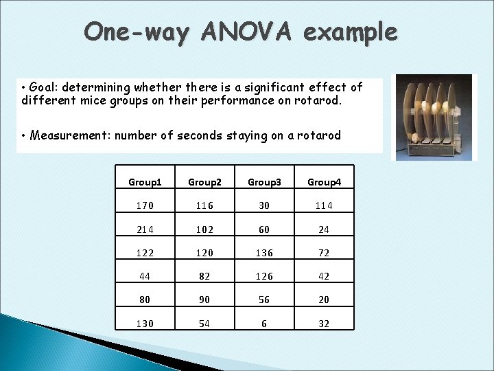
One-way ANOVA example • Goal: determining whethere is a significant effect of different mice groups on their performance on rotarod. • Measurement: number of seconds staying on a rotarod Group 1 Group 2 Group 3 Group 4 170 116 30 114 214 102 60 24 122 120 136 72 44 82 126 42 80 90 56 20 130 54 6 32

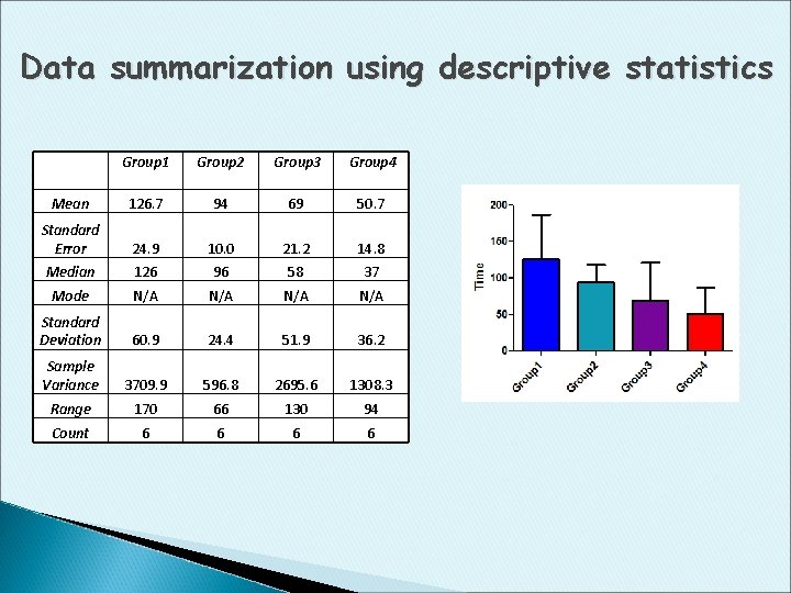
Data summarization using descriptive statistics Group 1 Group 2 Group 3 Group 4 Mean 126. 7 94 69 50. 7 Standard Error 24. 9 10. 0 21. 2 14. 8 Median 126 96 58 37 Mode N/A N/A Standard Deviation 60. 9 24. 4 51. 9 36. 2 Sample Variance 3709. 9 596. 8 2695. 6 1308. 3 Range 170 66 130 94 Count 6 6

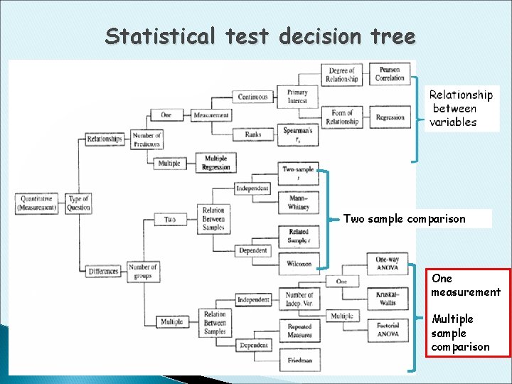
Statistical test decision tree Two sample comparison One measurement Multiple sample comparison

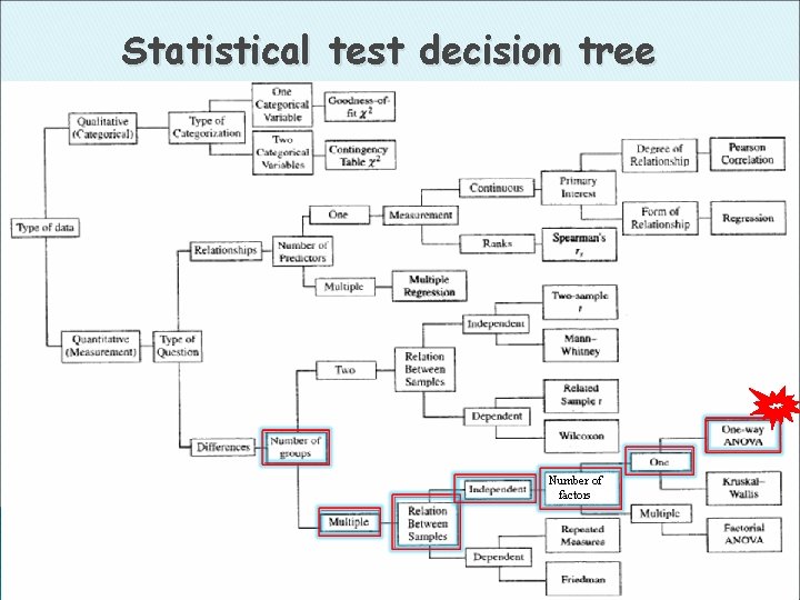
Statistical test decision tree Number of measurement Number of factors

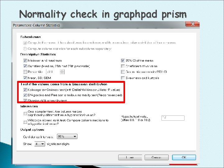
Normality check in graphpad prism

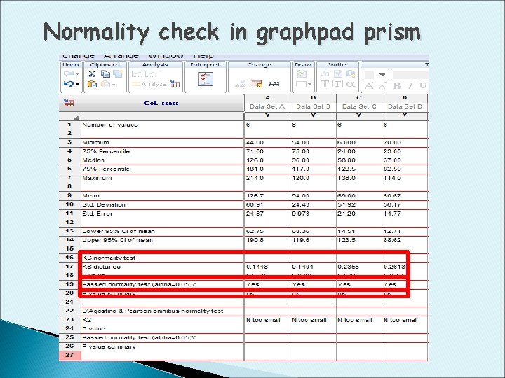
Normality check in graphpad prism

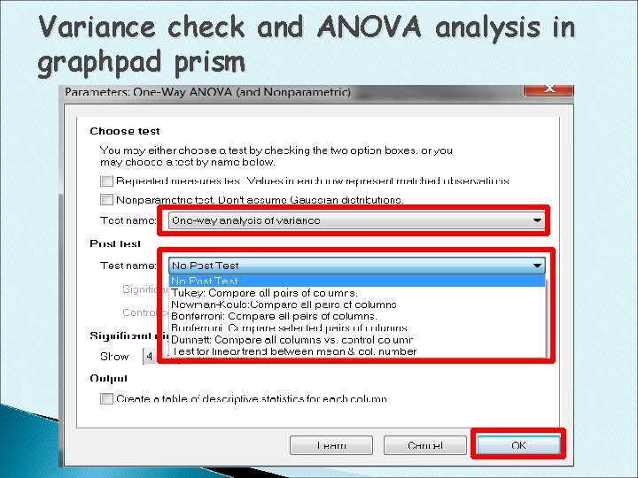
Variance check and ANOVA analysis in graphpad prism

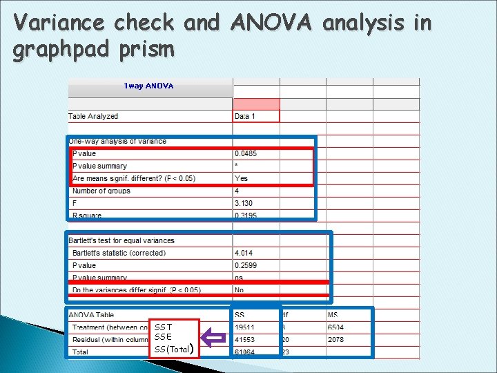
Variance check and ANOVA analysis in graphpad prism SST SSE SS(Total)

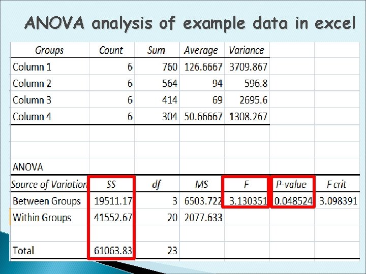
ANOVA analysis of example data in excel

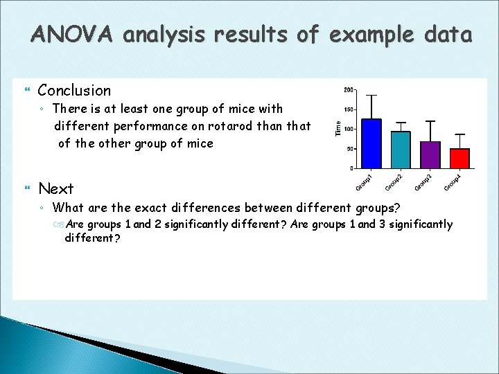
ANOVA analysis results of example data Conclusion ◦ There is at least one group of mice with different performance on rotarod than that of the other group of mice Next ◦ What are the exact differences between different groups? Are groups 1 and 2 significantly different? Are groups 1 and 3 significantly different?

Post hoc/multiple comparison tests introduction ANOVA does not differ groups from each other Problem of doing multiple t tests ◦ High combined false positive error rate 6 multiple t tests will give 26% chance of having at least one false positive error Multiple comparison tests ◦ They are based on T test or F test by considering the number of comparisons and adjust the p-value obtained from regular T test Pairwise comparisons ◦ Pairwise comparisons are differences between any two population means. On k populations or groups, there are k(k-1)/2 possible pairwise comparisons

Post hoc/multiple comparison tests introduction Error rate ◦ Familywise error rate(FWER) Probability of making at least one false positive among all the comparisons --Example: 4 groups, #of all possible pairwise comparisons=4(4 -1)/2=6 if the allowed false positive rate for each comparison is 0. 05, the probability of making at lease one false positive is 1 -(1 -0. 05) 6 =0. 26 control FWER at given α level such as 0. 05 ◦ False discovery rate (FDR) Used for large data sets such as microarray Probability of declared significant results that are actually false positives --Example: If 1000 genes were declared to have statistical significance, and FDR=0. 05, then 50 genes would be expected to be false positives Control FDR at given α level such as 0. 05

Common post hoc/multiple comparison tests Fisher’s protected least significant difference(fisher’s LSD) ◦ The first post hoc developed by Fisher to study pairwise comparisons ◦ Assumptions: equal variances, normality, and significant F test results ◦ Does not control FWER Tukey’s test ◦ Most popular post hoc and suitable for all pairwise comparisons (6 or more) ◦ Assumptions: equal variances and normality ◦ Control FWER and suitable for both equal and unequal sample size Bonferroni test ◦ Suitable for any set of preplanned comparison ◦ αper comparison= α/total number of comparisons ◦ Control FWER, too conservative in many situations

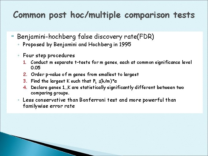
Common post hoc/multiple comparison tests Benjamini-hochberg false discovery rate(FDR) ◦ Proposed by Benjamini and Hochberg in 1995 ◦ Four step procedures 1. Conduct m separate t-tests for m genes, each at common significance level 0. 05 2. Order p-value of m genes from smallest to largest 3. Find the largest K such that Pk ≤(k/m)*α 4. Declare genes 1…K are statistically significantly different between two comparing groups. ◦ Less conservative than Bonferroni test and more powerful than familywise error rate

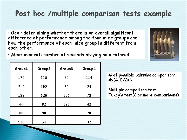
Post hoc /multiple comparison tests example • Goal: determining whethere is an overall significant difference of performance among the four mice groups and how the performance of each mice group is different from each other. • Measurement: number of seconds staying on a rotarod Group 1 Group 2 Group 3 Group 4 170 116 30 114 214 102 60 24 122 120 136 72 44 82 126 42 80 90 56 20 130 54 6 32 # of possible pairwise comparison: 4 x(4 -1)/2=6 Multiple comparison test: Tukey’s test(6 or more comparisons)

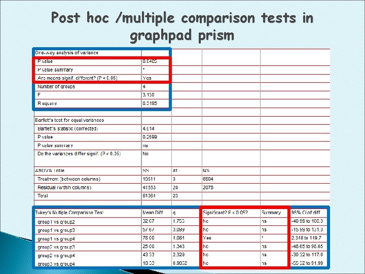
Post hoc /multiple comparison tests in graphpad prism

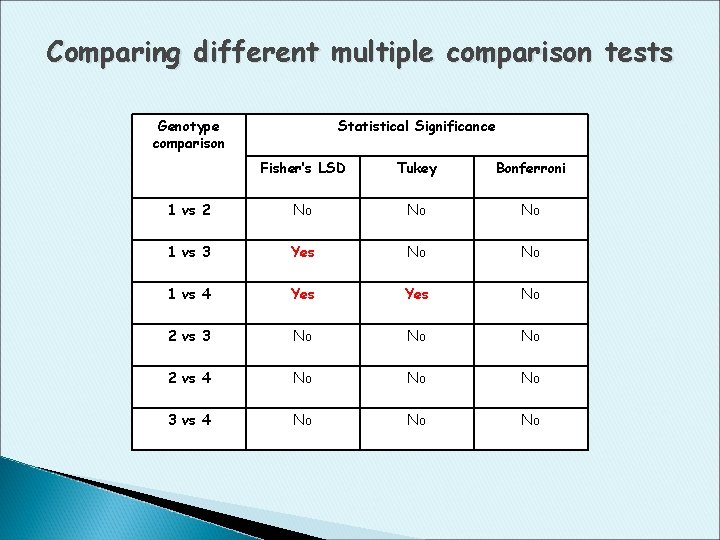
Comparing different multiple comparison tests Genotype comparison Statistical Significance Fisher’s LSD Tukey Bonferroni 1 vs 2 No No No 1 vs 3 Yes No No 1 vs 4 Yes No 2 vs 3 No No No 2 vs 4 No No No 3 vs 4 No No No

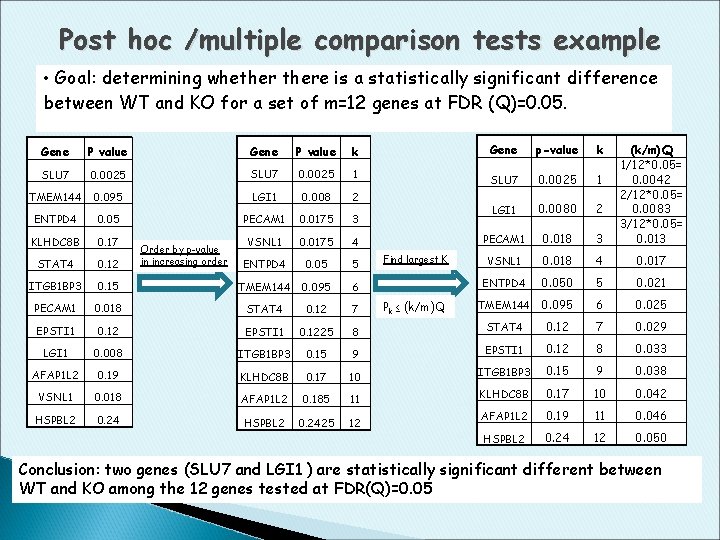
Post hoc /multiple comparison tests example • Goal: determining whethere is a statistically significant difference between WT and KO for a set of m=12 genes at FDR (Q)=0. 05. Gene p-value k SLU 7 0. 0025 1 LGI 1 0. 0080 2 PECAM 1 0. 018 3 (k/m)Q 1/12*0. 05= 0. 0042 2/12*0. 05= 0. 0083 3/12*0. 05= 0. 013 VSNL 1 0. 018 4 0. 017 ENTPD 4 0. 050 5 0. 021 TMEM 144 0. 095 6 0. 025 8 STAT 4 0. 12 7 0. 029 0. 15 9 EPSTI 1 0. 12 8 0. 033 KLHDC 8 B 0. 17 10 ITGB 1 BP 3 0. 15 9 0. 038 0. 018 AFAP 1 L 2 0. 185 11 KLHDC 8 B 0. 17 10 0. 042 0. 24 HSPBL 2 0. 2425 12 AFAP 1 L 2 0. 19 11 0. 046 HSPBL 2 0. 24 12 0. 050 Gene P value k SLU 7 0. 0025 1 TMEM 144 0. 095 LGI 1 0. 008 2 ENTPD 4 0. 05 PECAM 1 0. 0175 3 KLHDC 8 B 0. 17 VSNL 1 0. 0175 4 STAT 4 0. 12 ENTPD 4 0. 05 5 ITGB 1 BP 3 0. 15 TMEM 144 0. 095 6 PECAM 1 0. 018 STAT 4 0. 12 7 EPSTI 1 0. 1225 LGI 1 0. 008 ITGB 1 BP 3 AFAP 1 L 2 0. 19 VSNL 1 HSPBL 2 Order by p-value in increasing order Find largest K Pk ≤ (k/m)Q Conclusion: two genes (SLU 7 and LGI 1 ) are statistically significant different between WT and KO among the 12 genes tested at FDR(Q)=0. 05

Outline § Summary of Previous Talk ◦ Descriptive & inferential statistics ◦ T test § Common statistical tests and Applications (Continue) § One-way ANOVA § Post hoc/multiple comparison tests § One-way ANOVA power analysis § Common data transformation methods

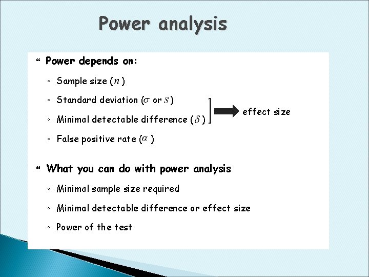
Power analysis Power depends on: ◦ Sample size ( ) ◦ Standard deviation ( or ) ◦ Minimal detectable difference ( ) effect size ◦ False positive rate ( ) What you can do with power analysis ◦ Minimal sample size required ◦ Minimal detectable difference or effect size ◦ Power of the test

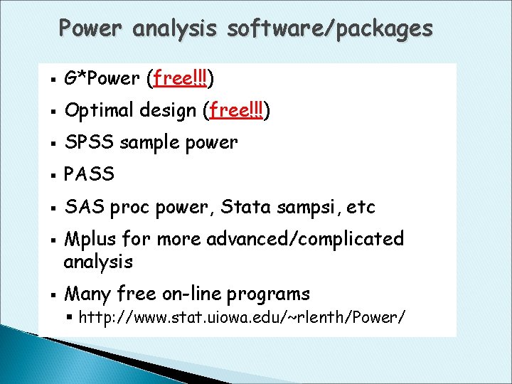
Power analysis software/packages § G*Power (free!!!) § Optimal design (free!!!) § SPSS sample power § PASS § SAS proc power, Stata sampsi, etc § § Mplus for more advanced/complicated analysis Many free on-line programs § http: //www. stat. uiowa. edu/~rlenth/Power/

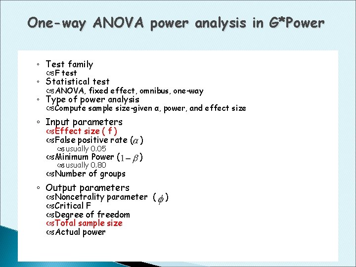
One-way ANOVA power analysis in G*Power ◦ Test family F test ◦ Statistical test ANOVA, fixed effect, omnibus, one-way ◦ Type of power analysis Compute sample size-given α, power, and effect size ◦ Input parameters Effect size ( f ) False positive rate ( ) usually 0. 05 Minimum Power ( usually 0. 80 ) Number of groups ◦ Output parameters Noncetrality parameter ( Critical F Degree of freedom Total sample size Actual power )

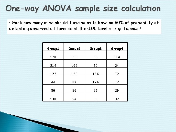
One-way ANOVA sample size calculation • Goal: how many mice should I use so as to have an 80% of probability of detecting observed difference at the 0. 05 level of significance? Group 1 Group 2 Group 3 Group 4 170 116 30 114 214 102 60 24 122 120 136 72 44 82 126 42 80 90 56 20 130 54 6 32

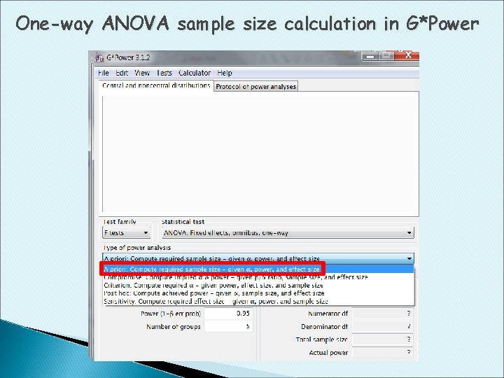
One-way ANOVA sample size calculation in G*Power

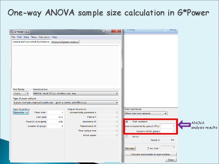
One-way ANOVA sample size calculation in G*Power ANOVA analysis results

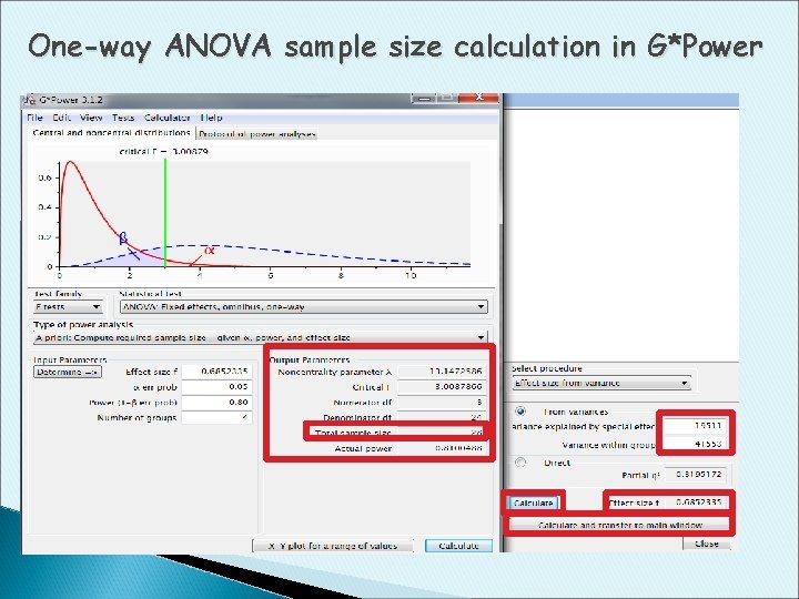
One-way ANOVA sample size calculation in G*Power

Outline § Summary of Previous Talk ◦ Descriptive & inferential statistics ◦ T test § Common statistical tests and Applications (Continue) § One-way ANOVA § Post hoc/multiple comparison tests § One-way ANOVA power analysis § Common data transformation methods

Data Transformation Why? ◦ Many biological variables do not follow normal distribution How? ◦ Applying a mathematical function on each observation ◦ Performing statistical tests using transformed data ◦ Interpreting results using back transformation Common data transformation methods in biology ◦ ◦ Log transformation Square root transformation Arcsine transformation Reciprocal transformation

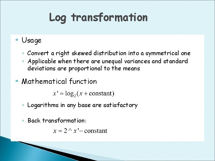
Log transformation Usage ◦ Convert a right skewed distribution into a symmetrical one ◦ Applicable when there are unequal variances and standard deviations are proportional to the means Mathematical function ◦ Logarithms in any base are satisfactory ◦ Back transformation:

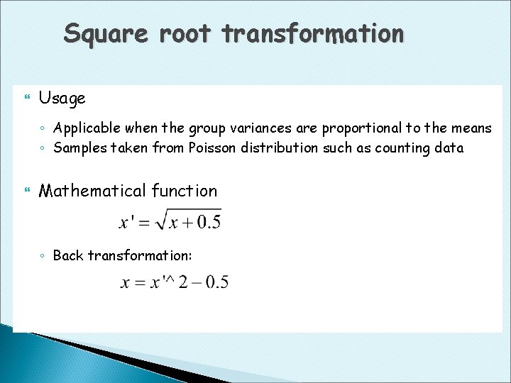
Square root transformation Usage ◦ Applicable when the group variances are proportional to the means ◦ Samples taken from Poisson distribution such as counting data Mathematical function ◦ Back transformation:

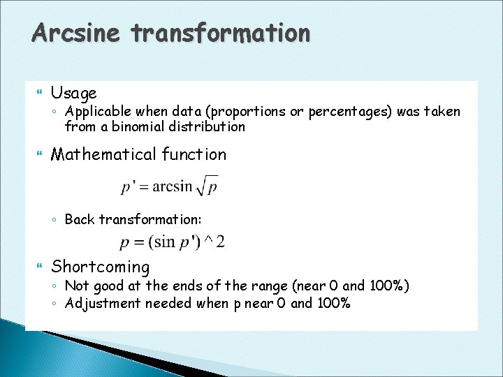
Arcsine transformation Usage ◦ Applicable when data (proportions or percentages) was taken from a binomial distribution Mathematical function ◦ Back transformation: Shortcoming ◦ Not good at the ends of the range (near 0 and 100%) ◦ Adjustment needed when p near 0 and 100%

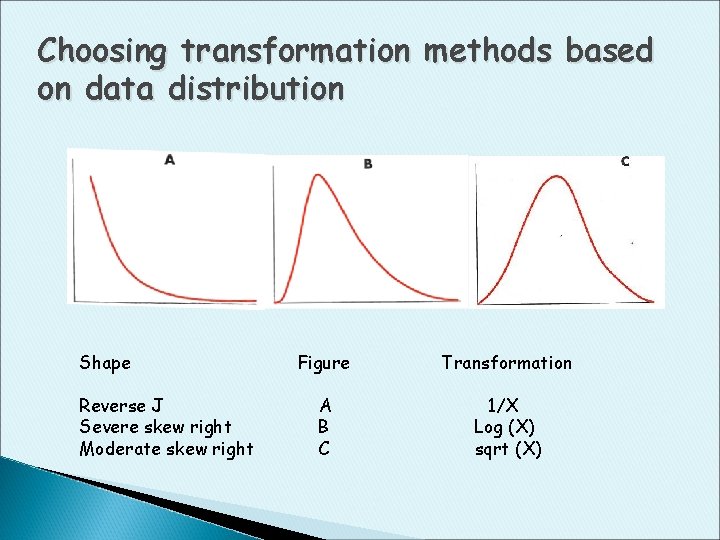
Choosing transformation methods based on data distribution Shape Reverse J Severe skew right Moderate skew right Figure Transformation A B C 1/X Log (X) sqrt (X)

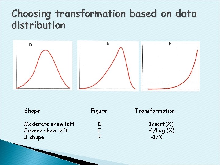
Choosing transformation based on data distribution Shape Moderate skew left Severe skew left J shape Figure D E F Transformation 1/sqrt(X) -1/Log (X) -1/X

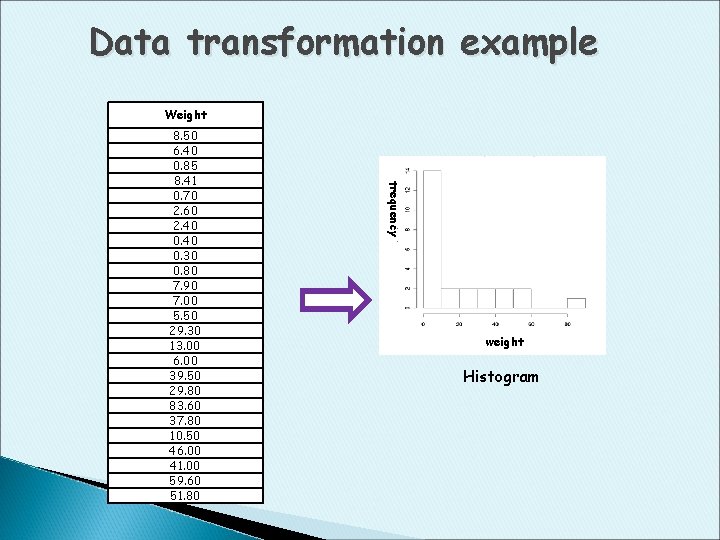
Data transformation example Weight frequency 8. 50 6. 40 0. 85 8. 41 0. 70 2. 60 2. 40 0. 30 0. 80 7. 90 7. 00 5. 50 29. 30 13. 00 6. 00 39. 50 29. 80 83. 60 37. 80 10. 50 46. 00 41. 00 59. 60 51. 80 weight Histogram

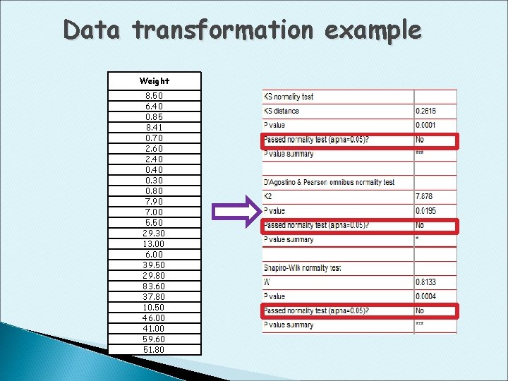
Data transformation example Weight 8. 50 6. 40 0. 85 8. 41 0. 70 2. 60 2. 40 0. 30 0. 80 7. 90 7. 00 5. 50 29. 30 13. 00 6. 00 39. 50 29. 80 83. 60 37. 80 10. 50 46. 00 41. 00 59. 60 51. 80

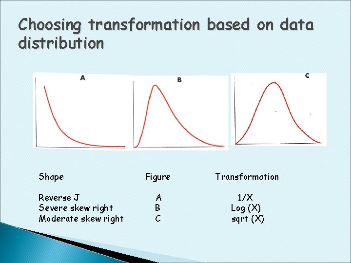
Choosing transformation based on data distribution Shape Reverse J Severe skew right Moderate skew right Figure Transformation A B C 1/X Log (X) sqrt (X)

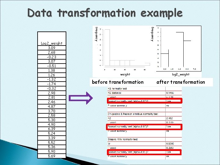
Data transformation example frequency Log 2_weight 3. 09 2. 68 -0. 23 3. 07 -0. 51 1. 38 1. 26 -1. 32 -1. 74 -0. 32 2. 98 2. 81 2. 46 4. 87 3. 70 2. 58 5. 30 4. 90 6. 39 5. 24 3. 39 5. 52 5. 36 5. 90 5. 69 weight before transformation log 2_weight after transformation

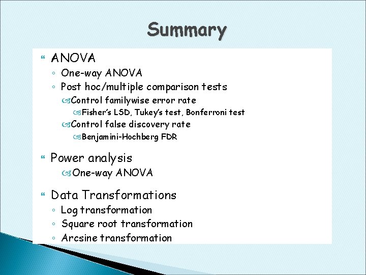
Summary ANOVA ◦ One-way ANOVA ◦ Post hoc/multiple comparison tests Control familywise error rate Fisher’s LSD, Tukey’s test, Bonferroni test Control false discovery rate Benjamini-Hochberg FDR Power analysis One-way ANOVA Data Transformations ◦ Log transformation ◦ Square root transformation ◦ Arcsine transformation

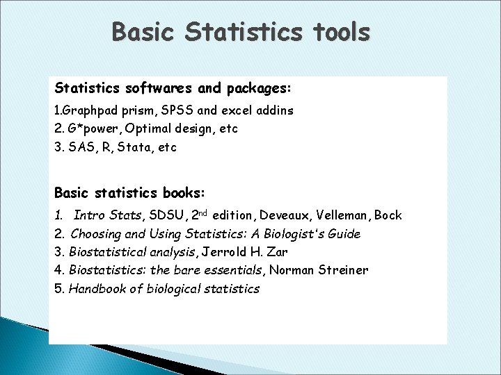
Basic Statistics tools Statistics softwares and packages: 1. Graphpad prism, SPSS and excel addins 2. G*power, Optimal design, etc 3. SAS, R, Stata, etc Basic statistics books: 1. Intro Stats, SDSU, 2 nd edition, Deveaux, Velleman, Bock 2. Choosing and Using Statistics: A Biologist's Guide 3. Biostatistical analysis, Jerrold H. Zar 4. Biostatistics: the bare essentials, Norman Streiner 5. Handbook of biological statistics

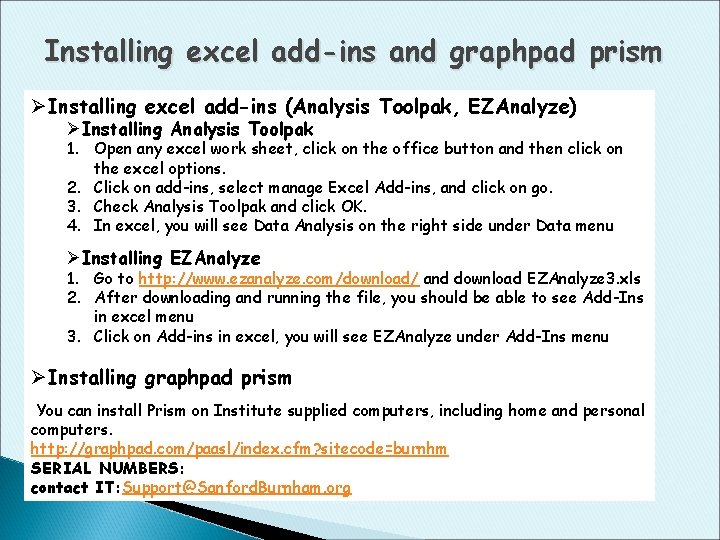
Installing excel add-ins and graphpad prism ØInstalling excel add-ins (Analysis Toolpak, EZAnalyze) ØInstalling Analysis Toolpak 1. Open any excel work sheet, click on the office button and then click on the excel options. 2. Click on add-ins, select manage Excel Add-ins, and click on go. 3. Check Analysis Toolpak and click OK. 4. In excel, you will see Data Analysis on the right side under Data menu ØInstalling EZAnalyze 1. Go to http: //www. ezanalyze. com/download/ and download EZAnalyze 3. xls 2. After downloading and running the file, you should be able to see Add-Ins in excel menu 3. Click on Add-ins in excel, you will see EZAnalyze under Add-Ins menu ØInstalling graphpad prism You can install Prism on Institute supplied computers, including home and personal computers. http: //graphpad. com/paasl/index. cfm? sitecode=burnhm SERIAL NUMBERS: contact IT: Support@Sanford. Burnham. org

Resources Many thanks for coming! My presentation will be posted on website: http: //bsrweb. burnham. org/ I am located in building 10, Office 2405, ext 3916 Feel free to come or call or send e-mail to ask questions (xyhuang@sanfordburnham. org)