Advanced Section 7 Decision trees and Ensemble methods

Advanced Section #7: Decision trees and Ensemble methods Camilo Fosco CS 109 A Introduction to Data Science Pavlos Protopapas and Kevin Rader 1

Outline • Decision trees • • Metrics Tree-building algorithms • Ensemble methods • • • Bagging Boosting Visualizations • Most common bagging techniques • Most common boosting techniques CS 109 A, PROTOPAPAS, RADER 2

DECISION TREES The backbone of most techniques 3

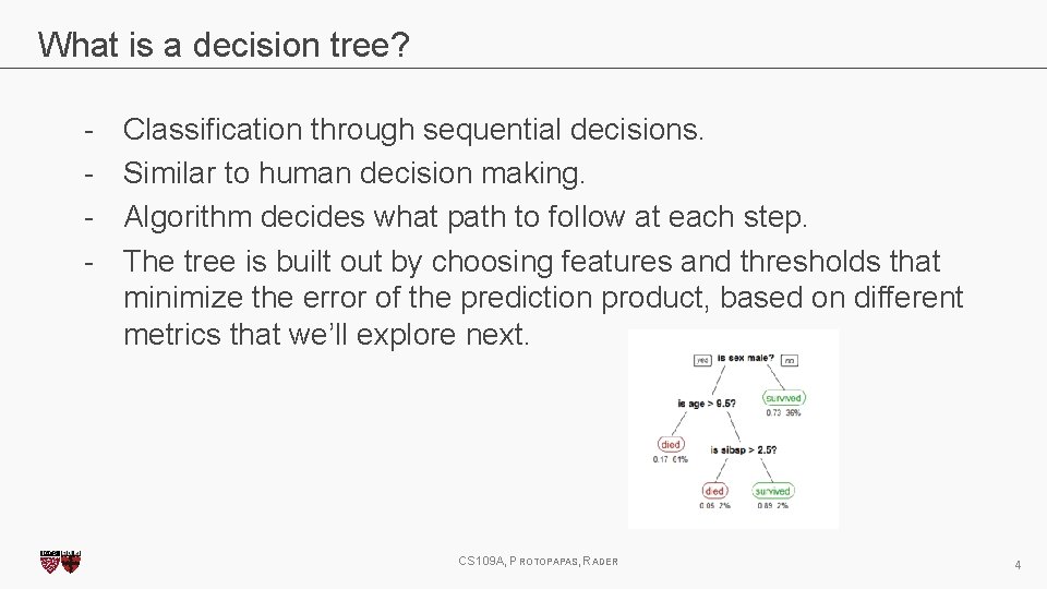
What is a decision tree? - Classification through sequential decisions. Similar to human decision making. Algorithm decides what path to follow at each step. The tree is built out by choosing features and thresholds that minimize the error of the prediction product, based on different metrics that we’ll explore next. CS 109 A, PROTOPAPAS, RADER 4

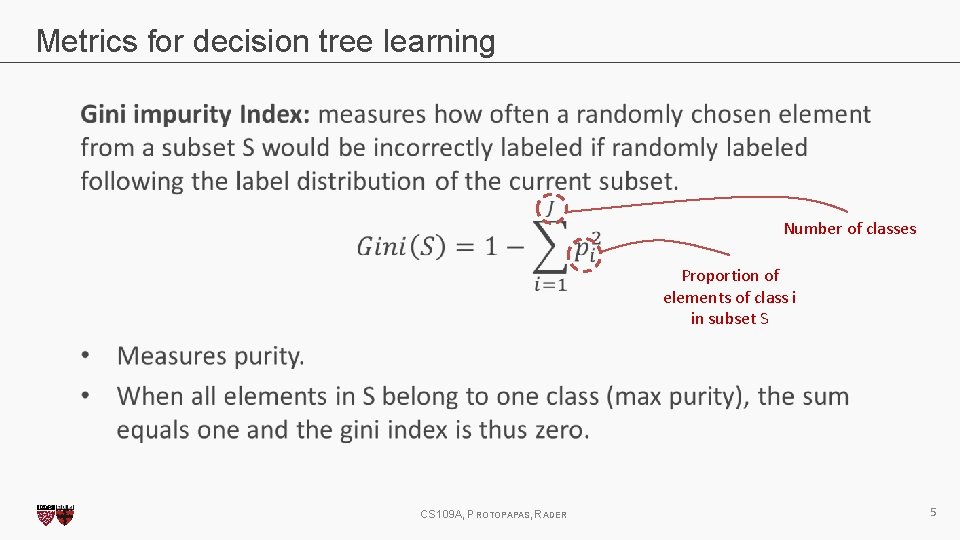
Metrics for decision tree learning Number of classes Proportion of elements of class i in subset S CS 109 A, PROTOPAPAS, RADER 5

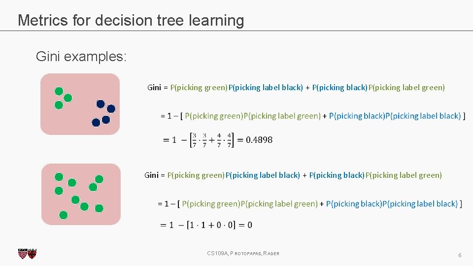
Metrics for decision tree learning Gini examples: Gini = P(picking green)P(picking label black) + P(picking black)P(picking label green) CS 109 A, PROTOPAPAS, RADER 6

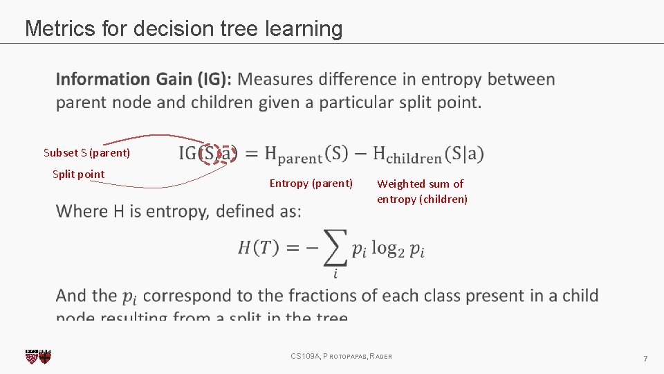
Metrics for decision tree learning Subset S (parent) Split point Entropy (parent) Weighted sum of entropy (children) CS 109 A, PROTOPAPAS, RADER 7

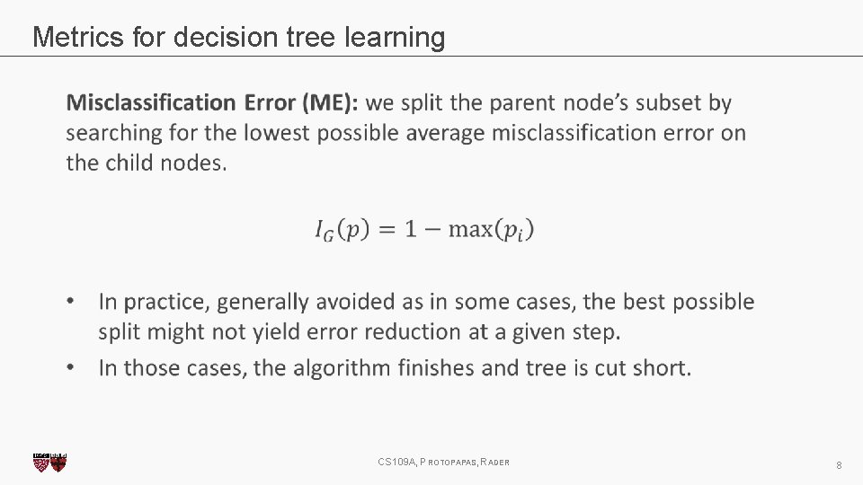
Metrics for decision tree learning CS 109 A, PROTOPAPAS, RADER 8

Tree-building algorithms ID 3: Iterative Dichotomiser 3. Developed in the 80 s by Ross Quinlan. • Uses the top-down induction approach described previously. • Works with the IG metric. • At each step, algorithm chooses feature to split on and calculates IG for each possible split along that feature. • Greedy algorithm. CS 109 A, PROTOPAPAS, RADER 9

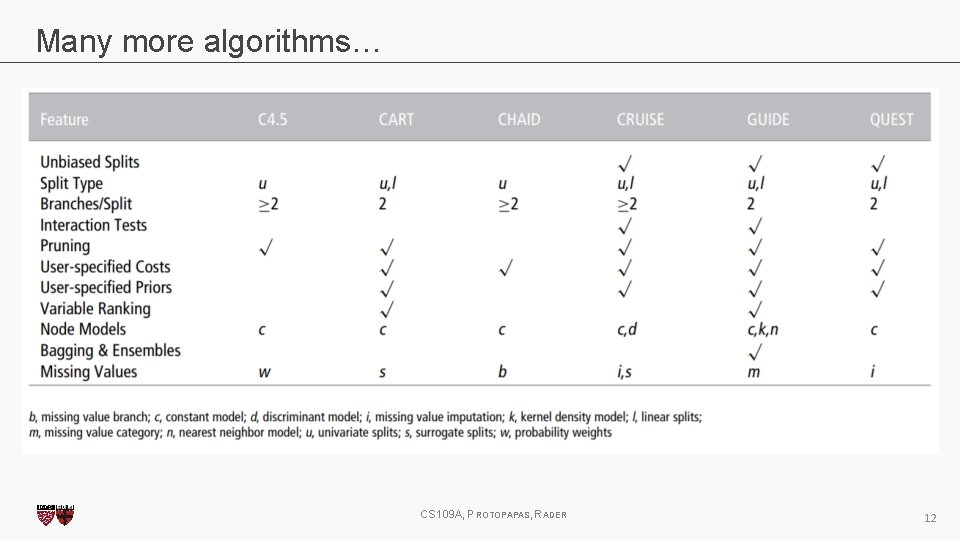
Tree-building algorithms C 4. 5: Successor of ID 3, also developed by Quinlan (‘ 93). Main improvements over I 3 D: • Works with both continuous and discrete features, while ID 3 only works with discrete values. • Handles missing values by using fractional cases (penalizes splits that have multiple missing values during training, fractionally assigns the datapoint to all possible outcomes). • Reduces overfitting by pruning, a bottom-up tree reduction technique. • Accepts weighting of input data. • Works with multiclass response variables. CS 109 A, PROTOPAPAS, RADER 10

Tree-building algorithms CART: Most popular tree-builder. Introduced by Breiman et al. in 1984. Usually used with Gini purity metric. • • • Main characteristic: builds binary trees. Can work with discrete, continuous and categorical values. Handles missing values by using surrogate splits. Uses cost-complexity pruning. Sklearn uses CART for its trees. CS 109 A, PROTOPAPAS, RADER 11

Many more algorithms… CS 109 A, PROTOPAPAS, RADER 12

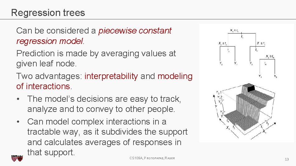
Regression trees Can be considered a piecewise constant regression model. Prediction is made by averaging values at given leaf node. Two advantages: interpretability and modeling of interactions. • The model’s decisions are easy to track, analyze and to convey to other people. • Can model complex interactions in a tractable way, as it subdivides the support and calculates averages of responses in that support. CS 109 A, PROTOPAPAS, RADER 13

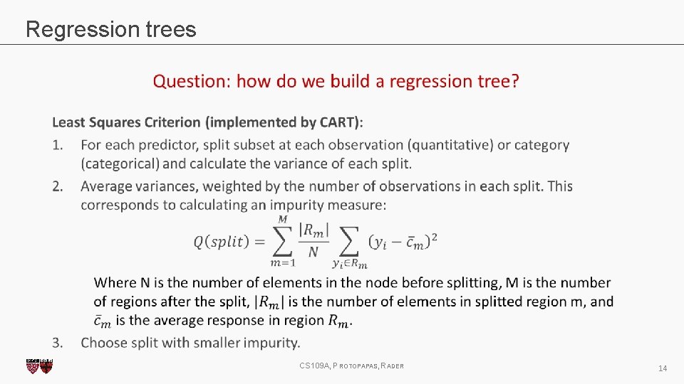
Regression trees CS 109 A, PROTOPAPAS, RADER 14

Regression trees - Cons Two major disadvantages: difficulty to capture simple relationships and instability. • Trees tend to have high variance. Small change in the data can produce a very different series of splits. • Any change at an upper level of the tree is propagated down the tree and affects all other splits. • Large number of splits necessary to accurately capture simple models such as linear and additive relationships. • Lack of smoothness. CS 109 A, PROTOPAPAS, RADER 15

Surrogate splits • When an observation is missing a value for predictor X, it cannot get past a node that splits based on this predictor. • We need surrogate splits: Mimic of original split in a node, but using another predictor. It is used in replacement of the original split in case a datapoint has missing data. • To build them, we search for a feature-threshold pair that most closely matches the original split. • “Association”: measure used to select surrogate splits. Depends on the probabilities of sending cases to a particular node + how the new split is separating observations of each class. CS 109 A, PROTOPAPAS, RADER 16

Surrogate splits • Two main functions: • • They split when the primary splitter is missing, which could never happen in the training data, but being ready for future test data increases robustness. They reveal common patterns among predictors in dataset. • No guarantee that useful surrogates can be found. • CART attempts to find at least 5 surrogates per node. • Number of surrogates usually varies from node to node. CS 109 A, PROTOPAPAS, RADER 17

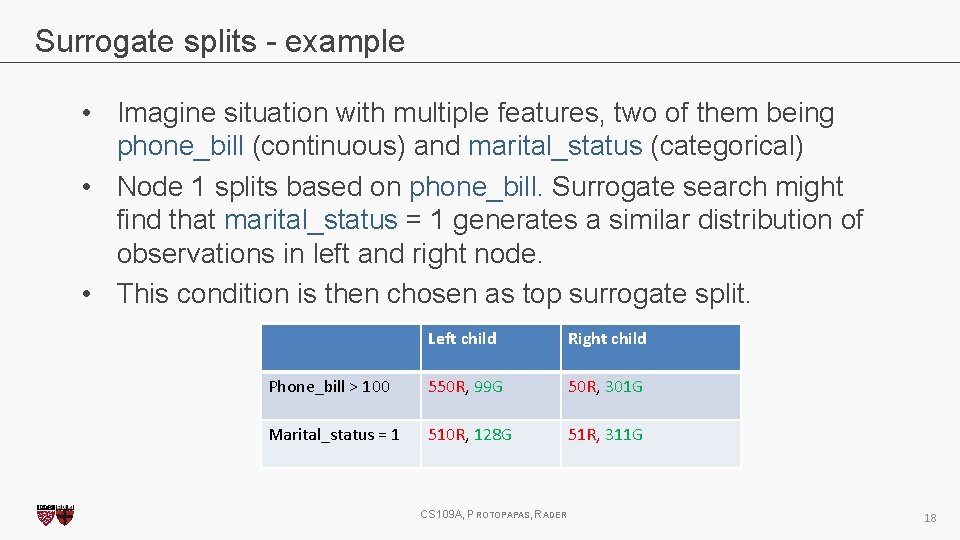
Surrogate splits - example • Imagine situation with multiple features, two of them being phone_bill (continuous) and marital_status (categorical) • Node 1 splits based on phone_bill. Surrogate search might find that marital_status = 1 generates a similar distribution of observations in left and right node. • This condition is then chosen as top surrogate split. Left child Right child Phone_bill > 100 649 550 R, 99 G 351 50 R, 301 G Marital_status = 1 638 510 R, 128 G 362 51 R, 311 G CS 109 A, PROTOPAPAS, RADER 18

Surrogate splits - example • In our example, primary splitter = phone_bill • We might find that surrogate splits include marital status, commute time, age, city of residence. • • • Commute time associated with more time on the phone Older individuals might be more likely to call vs text City variable hard to interpret because we don’t know identity of cities • Surrogates can help us understand primary splitter. CS 109 A, PROTOPAPAS, RADER 19

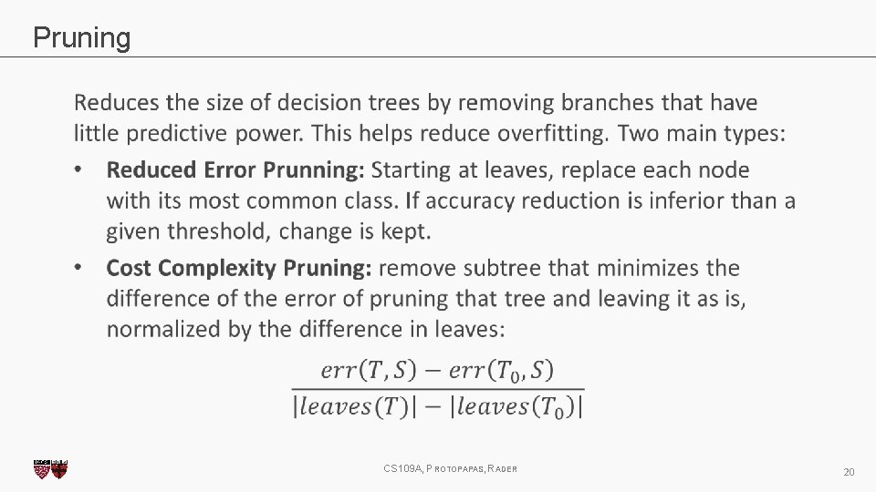
Pruning CS 109 A, PROTOPAPAS, RADER 20

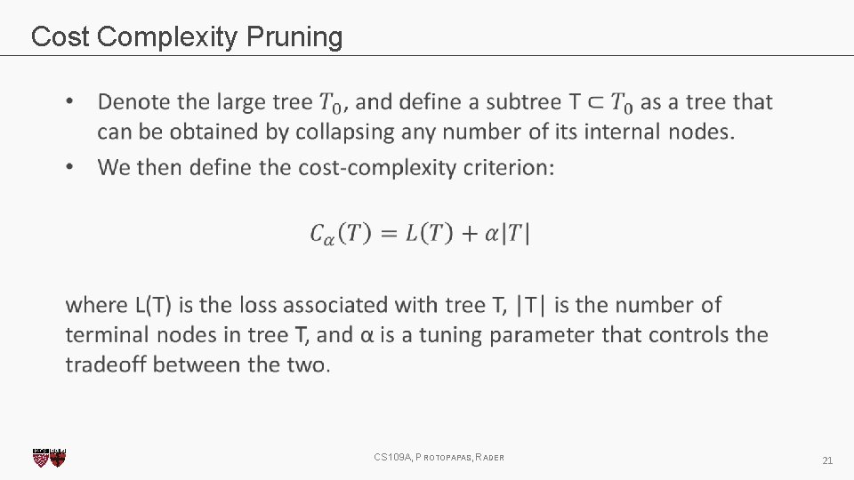
Cost Complexity Pruning CS 109 A, PROTOPAPAS, RADER 21

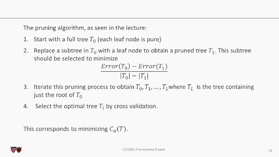
CS 109 A, PROTOPAPAS, RADER 22

ENSEMBLE METHODS Assemblers 2: Age of weak learners 23

What are ensemble methods? • Combination of weak learners to increase accuracy and reduce overfitting. • Train multiple models with a common objective and fuse their outputs. Multiple ways of fusing them, can you think of some? • Main causes of error in learning: noise, bias, variance. Ensembles help reduce those factors. • Improves stability of machine learning models. Combination of multiple learners reduces variance, especially in the case of unstable classifiers. CS 109 A, PROTOPAPAS, RADER 24

What are ensemble methods? • Typically, decision trees are used as base learners. • Ensembles usually retrain learners on subsets of the data. • Multiple ways to get those subsets: • • Resample original data with replacement: Bagging. Resample original data by choosing troublesome points more often: Boosting. • The learners can also be retrained on modified versions of the original data (gradient boosting). CS 109 A, PROTOPAPAS, RADER 25

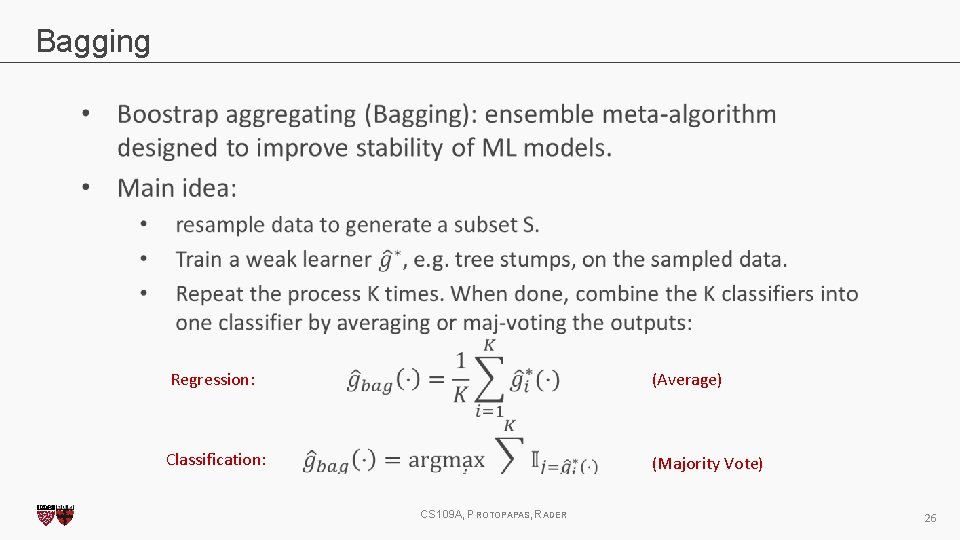
Bagging Regression: (Average) Classification: (Majority Vote) CS 109 A, PROTOPAPAS, RADER 26

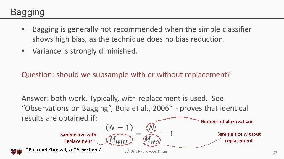
Bagging Number of observations Sample size without replacement Sample size with replacement *Buja and Stuetzel, 2006, section 7. CS 109 A, PROTOPAPAS, RADER 27

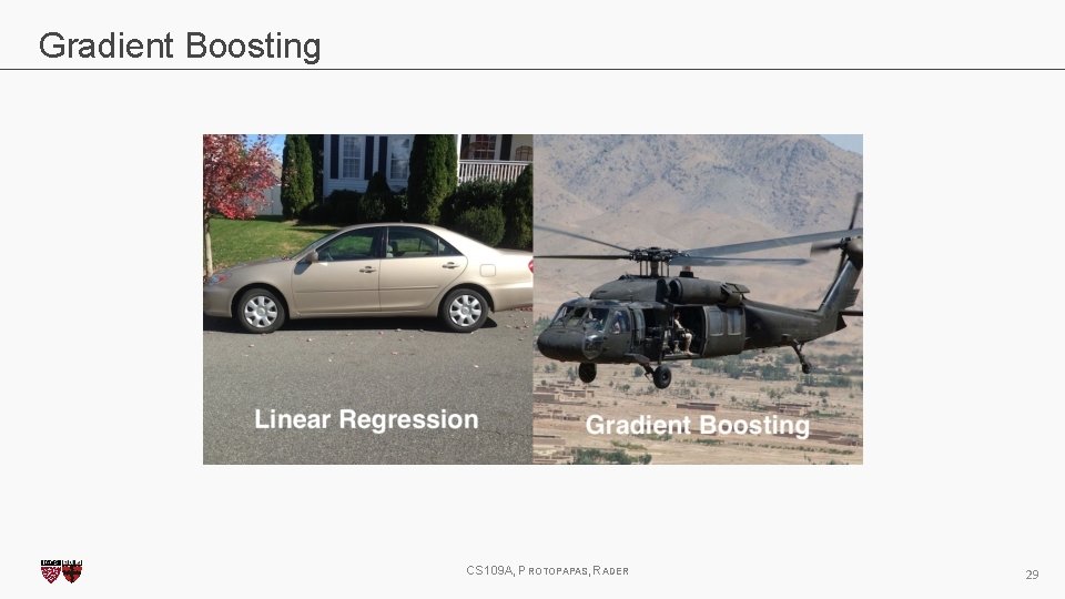
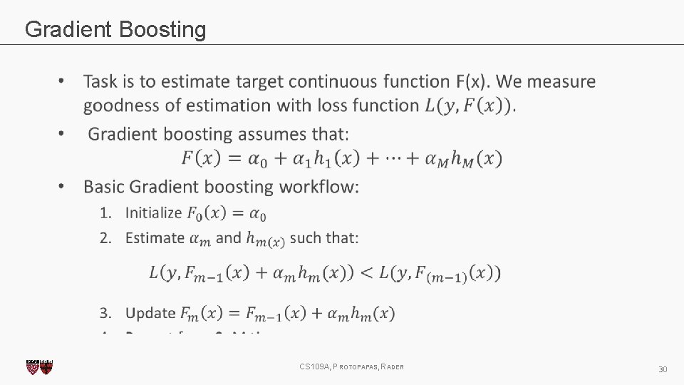
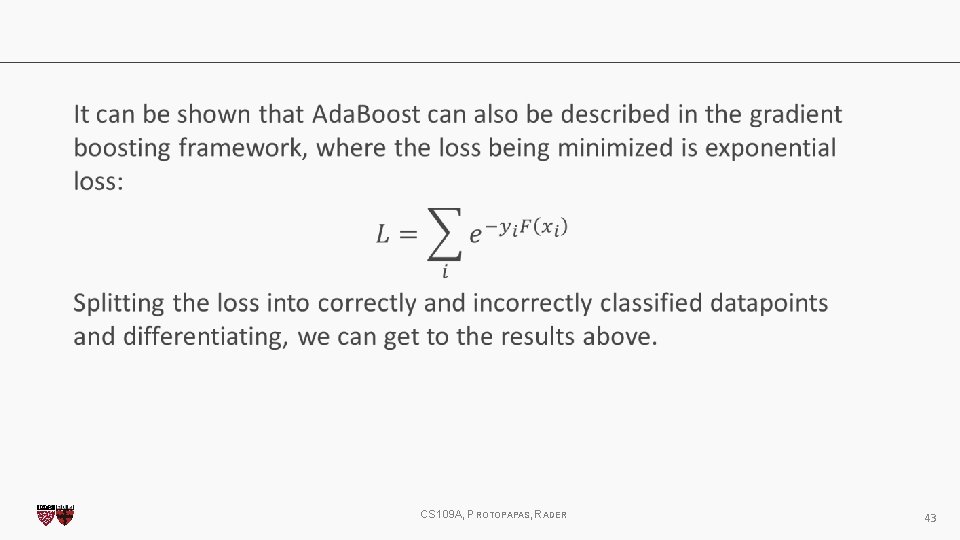
Boosting • Sequential algorithm where at each step, a weak learner is trained based on the results of the previous learner. • Two main types: • • Adaptive Boosting: Reweight datapoints based on performance of last weak learner. Focuses on points where previous learner had trouble. Example: Ada. Boost. Gradient Boosting: Train new learner on residuals of overall model. Constitutes gradient boosting because approximating the residual and adding to the previous result is essentially a form of gradient descent. Example: XGBoost. CS 109 A, PROTOPAPAS, RADER 28

Gradient Boosting CS 109 A, PROTOPAPAS, RADER 29

Gradient Boosting CS 109 A, PROTOPAPAS, RADER 30

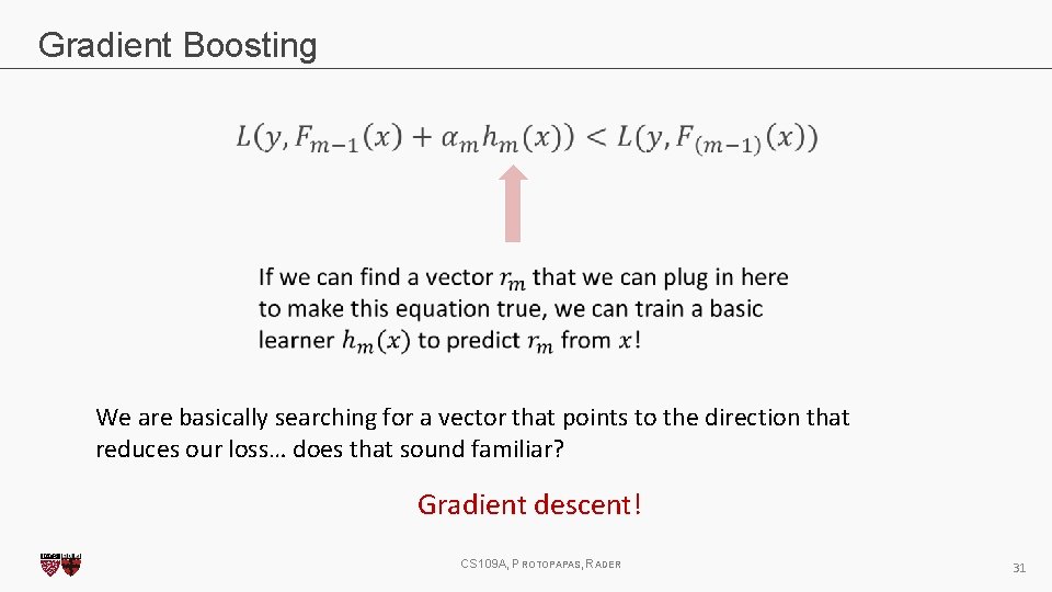
Gradient Boosting We are basically searching for a vector that points to the direction that reduces our loss… does that sound familiar? Gradient descent! CS 109 A, PROTOPAPAS, RADER 31

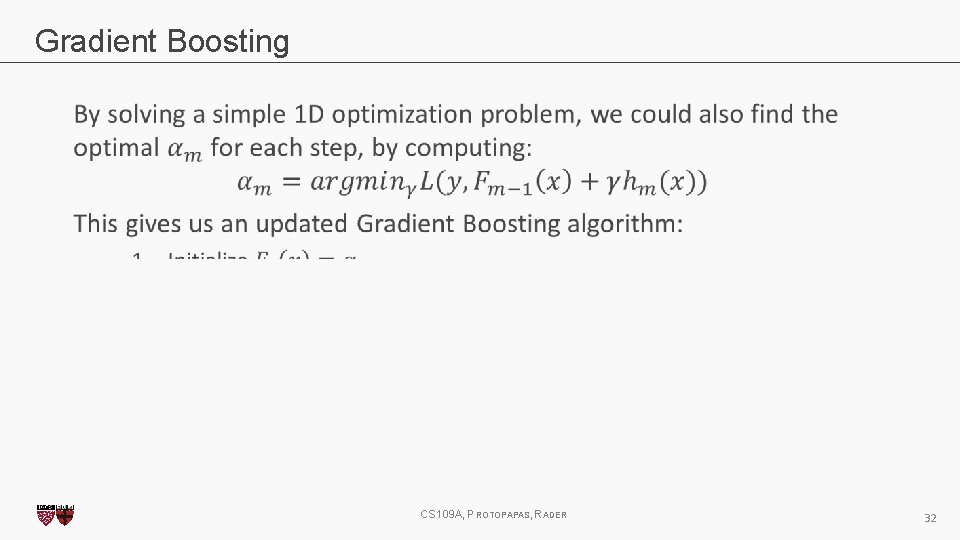
Gradient Boosting CS 109 A, PROTOPAPAS, RADER 32

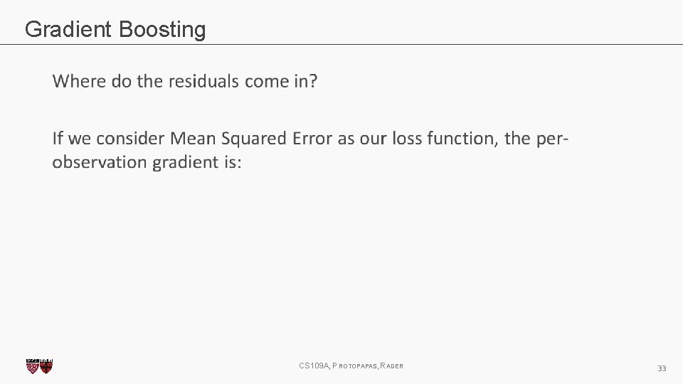
Gradient Boosting CS 109 A, PROTOPAPAS, RADER 33

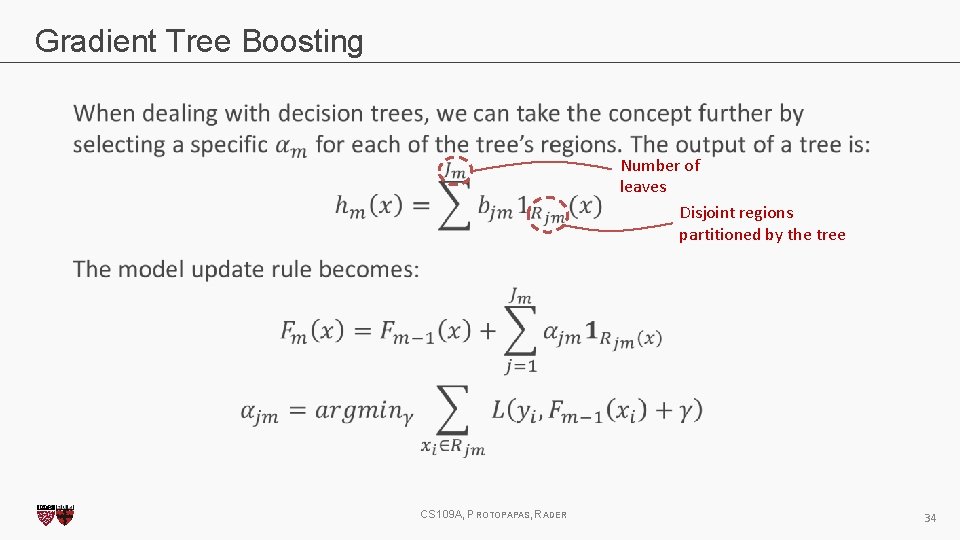
Gradient Tree Boosting Number of leaves Disjoint regions partitioned by the tree CS 109 A, PROTOPAPAS, RADER 34

Let’s look at graphs! GRAPH TIME http: //arogozhnikov. github. io/2016/06/24/gradient_boosting_explained. html CS 109 A, PROTOPAPAS, RADER 35

COMMON BAGGING TECHNIQUES Random Forests, of course. 36

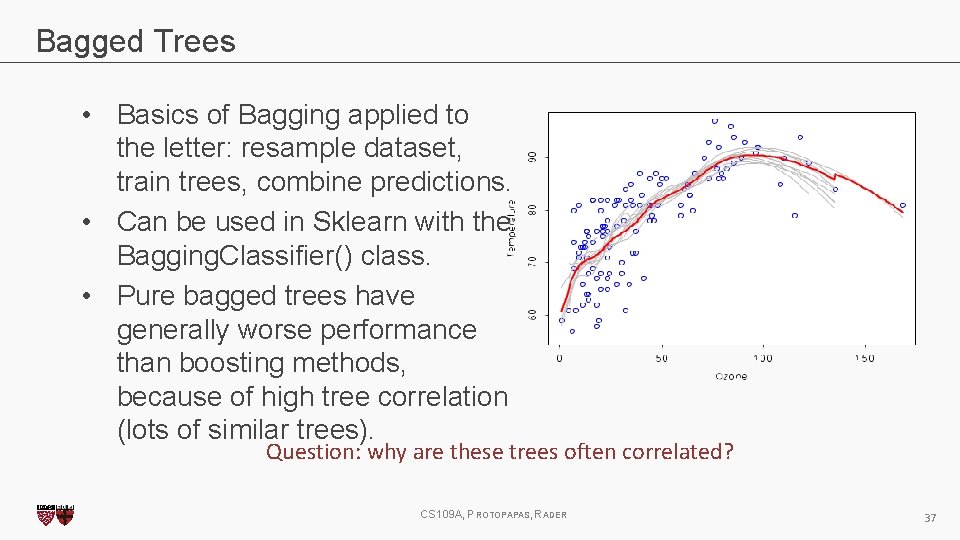
Bagged Trees • Basics of Bagging applied to the letter: resample dataset, train trees, combine predictions. • Can be used in Sklearn with the Bagging. Classifier() class. • Pure bagged trees have generally worse performance than boosting methods, because of high tree correlation (lots of similar trees). Question: why are these trees often correlated? CS 109 A, PROTOPAPAS, RADER 37

Random Forests • Similar to bagged trees but with a twist: we now choose a random subset of predictors when defining our trees. • Question: Do we choose a random subset for each tree, or for each node? • Random Forests essentially perform bagging over the predictor space and build a collection of de-correlated trees. • This increases the stability of the algorithm and tackles correlation problems that arise by a greedy search of the best split at each node. • Adds diversity, reduces variance of total estimator at the cost of an equal or higher bias. CS 109 A, PROTOPAPAS, RADER 38

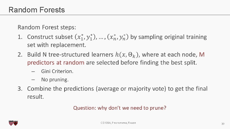
Random Forests Question: why don’t we need to prune? CS 109 A, PROTOPAPAS, RADER 39

COMMON BOOSTING TECHNIQUES Kaggle killers. 40

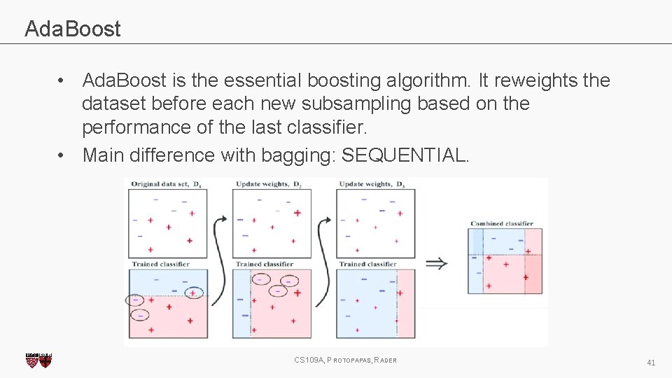
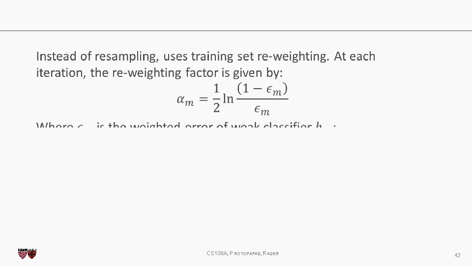
Ada. Boost • Ada. Boost is the essential boosting algorithm. It reweights the dataset before each new subsampling based on the performance of the last classifier. • Main difference with bagging: SEQUENTIAL. CS 109 A, PROTOPAPAS, RADER 41

CS 109 A, PROTOPAPAS, RADER 42

CS 109 A, PROTOPAPAS, RADER 43

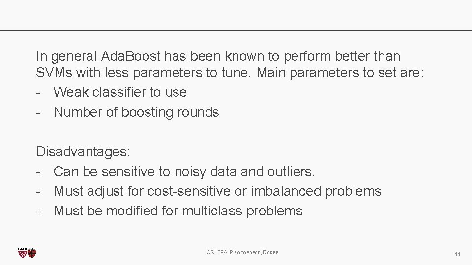
In general Ada. Boost has been known to perform better than SVMs with less parameters to tune. Main parameters to set are: - Weak classifier to use - Number of boosting rounds Disadvantages: - Can be sensitive to noisy data and outliers. - Must adjust for cost-sensitive or imbalanced problems - Must be modified for multiclass problems CS 109 A, PROTOPAPAS, RADER 44

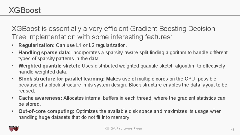
XGBoost is essentially a very efficient Gradient Boosting Decision Tree implementation with some interesting features: • Regularization: Can use L 1 or L 2 regularization. • Handling sparse data: Incorporates a sparsity-aware split finding algorithm to handle different types of sparsity patterns in the data. • Weighted quantile sketch: Uses distributed weighted quantile sketch algorithm to effectively handle weighted data. • Block structure for parallel learning: Makes use of multiple cores on the CPU, possible because of a block structure in its system design. Block structure enables the data layout to be reused. • Cache awareness: Allocates internal buffers in each thread, where the gradient statistics can be stored. • Out-of-core computing: Optimizes the available disk space and maximizes its usage when handling huge datasets that do not fit into memory. CS 109 A, PROTOPAPAS, RADER 45

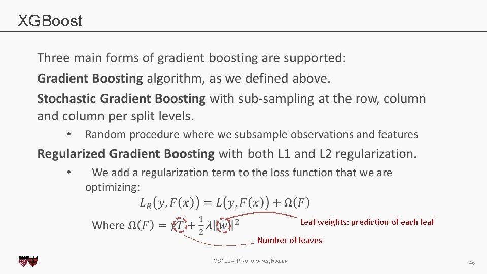
XGBoost Leaf weights: prediction of each leaf Number of leaves CS 109 A, PROTOPAPAS, RADER 46

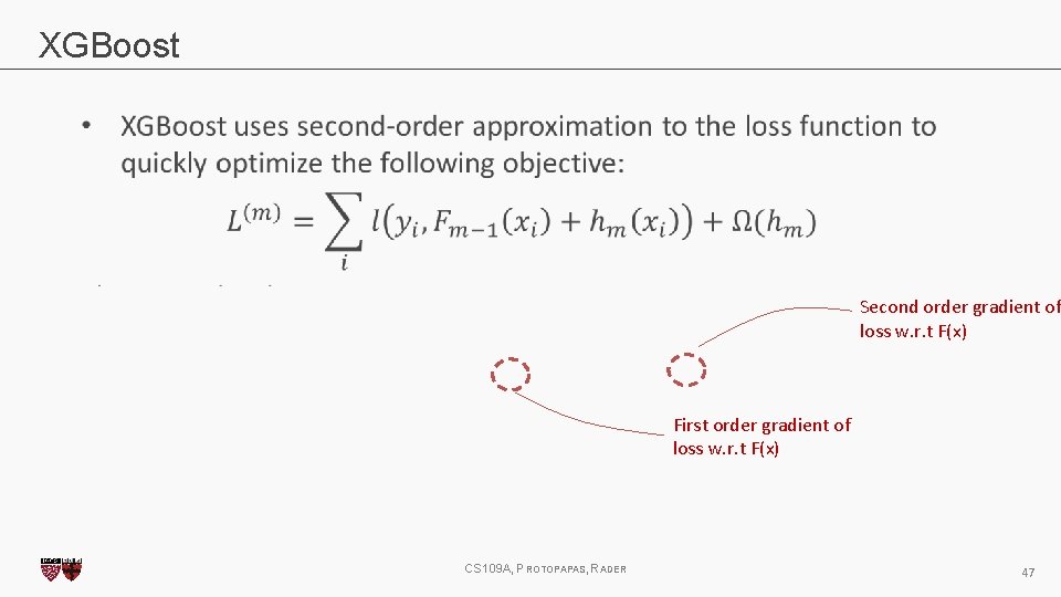
XGBoost Second order gradient of loss w. r. t F(x) First order gradient of loss w. r. t F(x) CS 109 A, PROTOPAPAS, RADER 47

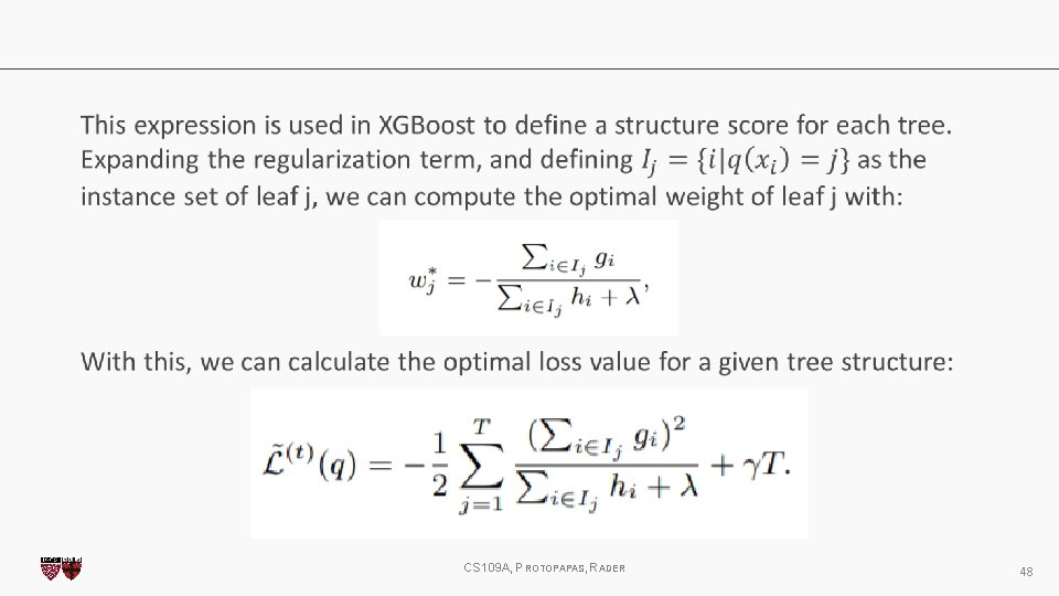
CS 109 A, PROTOPAPAS, RADER 48

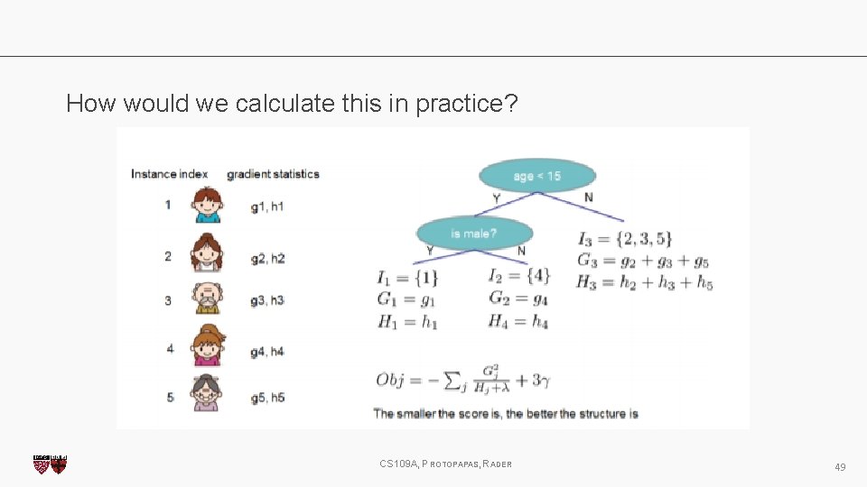
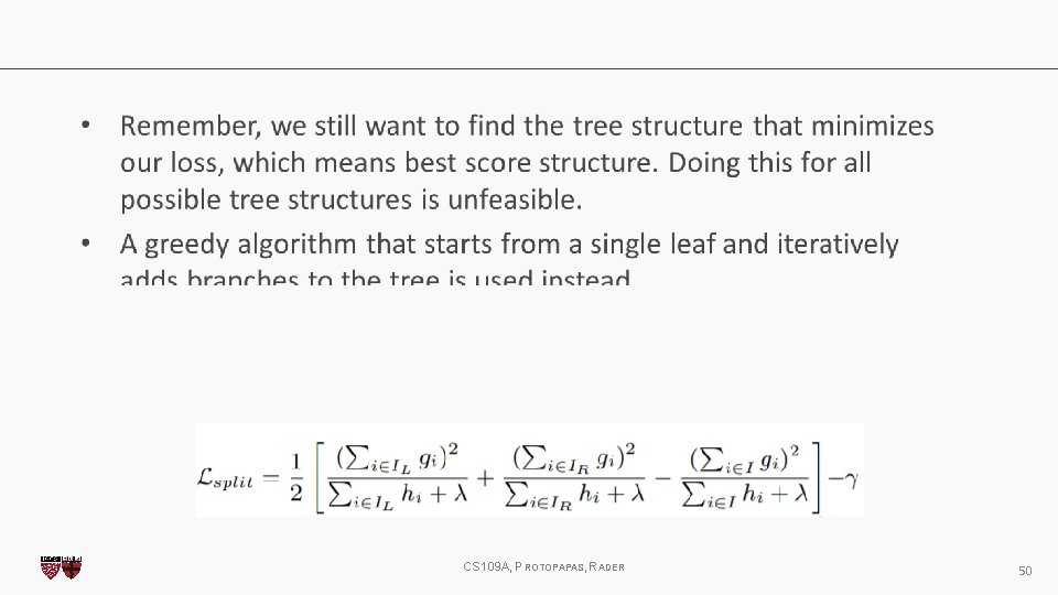
How would we calculate this in practice? CS 109 A, PROTOPAPAS, RADER 49

CS 109 A, PROTOPAPAS, RADER 50

XGBoost adds multiple other important advancements that make it state of the art in several industrial applications. In practice: - Can take a while to run if you don’t set the n_jobs parameter correctly - Defining the eta parameter (analogous to learning rate) and max_depth is crucial to obtain good performance. - Alpha parameter controls L 1 regularization, can be increased on high dimensionality problems to increase run time. CS 109 A, PROTOPAPAS, RADER 51

General approach to parameter tuning: • • Cross-validate learning rate. Determine the optimum number of trees for this learning rate. XGBoost can perform cross-validation at each boosting iteration for this, with the “cv” function. Tune tree-specific parameters (max_depth, min_child_weight, gamma, subsample, colsample_bytree) for chosen learning rate and number of trees. Tune regularization parameters (lambda, alpha). CS 109 A, PROTOPAPAS, RADER 52

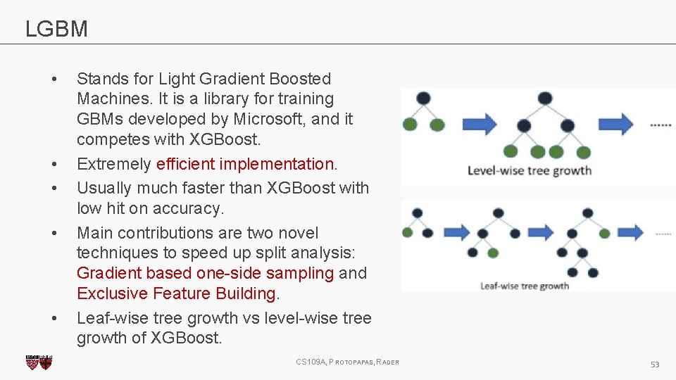
LGBM • • • Stands for Light Gradient Boosted Machines. It is a library for training GBMs developed by Microsoft, and it competes with XGBoost. Extremely efficient implementation. Usually much faster than XGBoost with low hit on accuracy. Main contributions are two novel techniques to speed up split analysis: Gradient based one-side sampling and Exclusive Feature Building. Leaf-wise tree growth vs level-wise tree growth of XGBoost. CS 109 A, PROTOPAPAS, RADER 53

Gradient-based one-side sampling (GOSS) • Normally, no native weight for datapoints, but in can be seen that instances with larger gradients (i. e. , under-trained instances) will contribute more to the information gain metric. • LGBM keeps instances with large gradients and only randomly drops instances with small gradients when subsampling. • They prove that this can lead to a more accurate gain estimation than uniformly random sampling, with the same target sampling rate, especially when the value of information gain has a large range. CS 109 A, PROTOPAPAS, RADER 54

Exclusive Feature Bundling (EFB) • Usually, feature space is quite sparse. • Specifically, in a sparse feature space, many features are (almost) exclusive, i. e. , they rarely take nonzero values simultaneously. Examples include one-hot encoded-features. • LGBM bundles those features by reducing the optimal bundling problem to a graph coloring problem (by taking features as vertices and adding edges for every two features if they are not mutually exclusive), and solving it by a greedy algorithm with a constant approximation ratio. CS 109 A, PROTOPAPAS, RADER 55

Cat. Boost • A new library for Gradient Boosting Decision Trees, offering appropriate handling of categorical features. • Presented as a workshop at NIPS 2017. • Fast, scalable and high-performance. Outperforms LGBM and XGBoost on inference times, and in some datasets, in accuracy as well. • Main idea: deal with categorical variables by using random permutations of the dataset and calculating the average label value for a given example using the label values of previous examples with the same category. CS 109 A, PROTOPAPAS, RADER 56

THANK YOU! 57

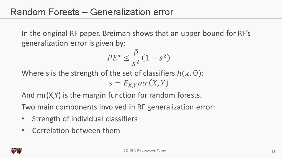
Random Forests – Generalization error CS 109 A, PROTOPAPAS, RADER 58