Advanced Programming Handout 6 Purely Functional Data Structures

Advanced Programming Handout 6 Purely Functional Data Structures: A Case Study in Functional Programming

Persistent vs. Ephemeral An ephemeral data structure is one for which only one version is available at a time: after an update operation, the structure as it existed before the update is lost. n A persistent structure is one where multiple versions are simultaneously accessible: after an update, both old and new versions can be used. n

Persistent vs. Ephemeral n In imperative languages, most data structures are ephemeral. • It is generally accepted that persistent variants, when they are possible at all, will be more complex to code and asymptotically less efficient. n In purely functional languages like Haskell, all data structures are persistent! • Since there is no assignment, there is no way to destroy old information. When we are done with it, we just drop it on the floor and let the garbage collector take care of it. n So one might worry that efficient data structures might be hard or even impossible to code in Haskell.

Enter Okasaki n n Interestingly, it turns out that many common data structures have purely functional variants that are easy to understand have exacly the same asymptotic efficiency as their imperative, ephemeral variants. These structures have been explored in an influential book, Purely Functional Data Structures, by Chris Okasaki, and in a long series of research papers by Okasaki and others.

Simple Example n To get started, let’s take a quite simple trick that was known to functional programmers long before Okasaki. . .

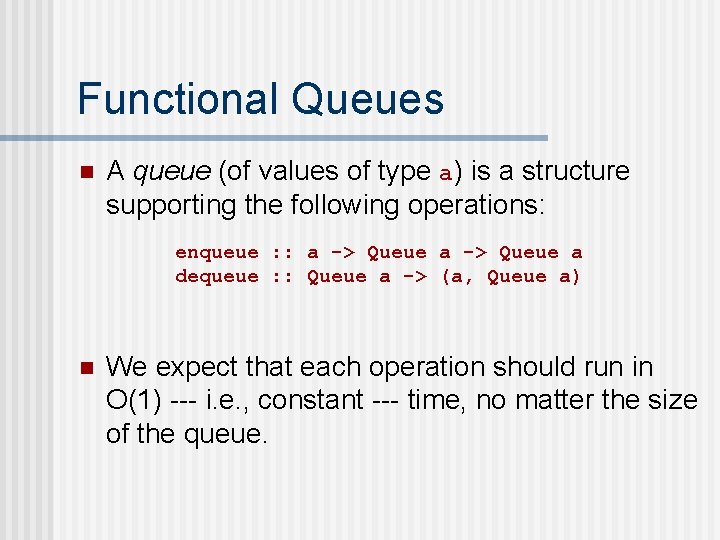
Functional Queues n A queue (of values of type a) is a structure supporting the following operations: enqueue : : a -> Queue a dequeue : : Queue a -> (a, Queue a) n We expect that each operation should run in O(1) --- i. e. , constant --- time, no matter the size of the queue.

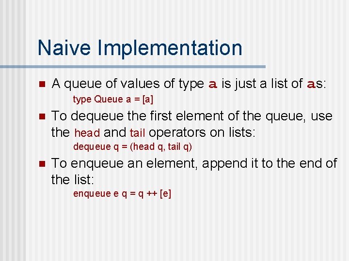
Naive Implementation n A queue of values of type a is just a list of as: type Queue a = [a] n To dequeue the first element of the queue, use the head and tail operators on lists: dequeue q = (head q, tail q) n To enqueue an element, append it to the end of the list: enqueue e q = q ++ [e]

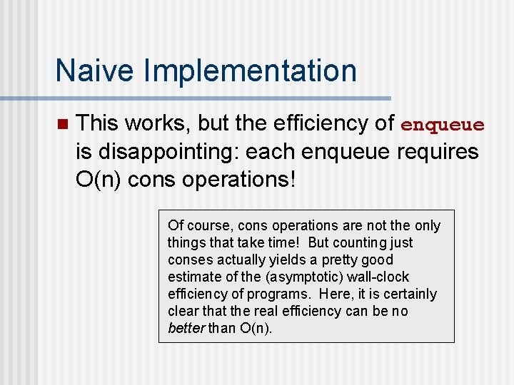
Naive Implementation n This works, but the efficiency of enqueue is disappointing: each enqueue requires O(n) cons operations! Of course, cons operations are not the only things that take time! But counting just conses actually yields a pretty good estimate of the (asymptotic) wall-clock efficiency of programs. Here, it is certainly clear that the real efficiency can be no better than O(n).

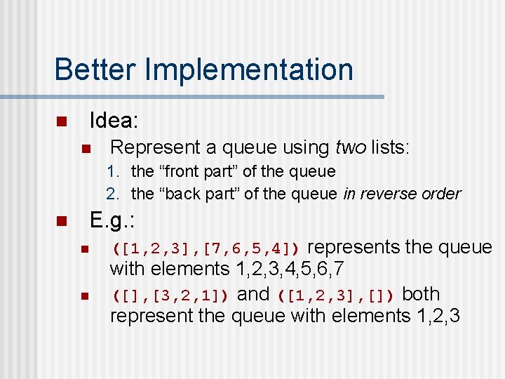
Better Implementation n Idea: n Represent a queue using two lists: 1. the “front part” of the queue 2. the “back part” of the queue in reverse order n E. g. : n n ([1, 2, 3], [7, 6, 5, 4]) represents the queue with elements 1, 2, 3, 4, 5, 6, 7 ([], [3, 2, 1]) and ([1, 2, 3], []) both represent the queue with elements 1, 2, 3

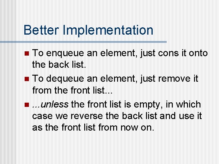
Better Implementation To enqueue an element, just cons it onto the back list. n To dequeue an element, just remove it from the front list. . . n. . . unless the front list is empty, in which case we reverse the back list and use it as the front list from now on. n

Better Implementation data Queue a = Queue [a] enqueue : : a -> Queue a enqueue e (Queue front back) = Queue front (e: back) dequeue : : Queue a -> (a, Queue a) dequeue (Queue (e: front) back) = (e, (Queue front back)) dequeue (Queue [] back) = dequeue (Queue (reverse back) [])

Efficiency n Intuition: a dequeue may require O(n) cons operations (to reverse the back list), but this cannot happen too often.

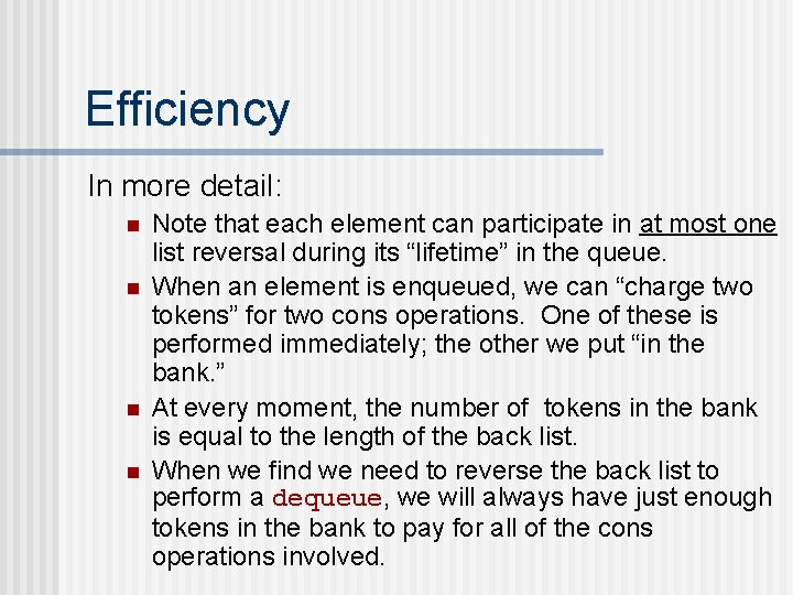
Efficiency In more detail: n n Note that each element can participate in at most one list reversal during its “lifetime” in the queue. When an element is enqueued, we can “charge two tokens” for two cons operations. One of these is performed immediately; the other we put “in the bank. ” At every moment, the number of tokens in the bank is equal to the length of the back list. When we find we need to reverse the back list to perform a dequeue, we will always have just enough tokens in the bank to pay for all of the cons operations involved.

Efficiency So we can say that the amortized cost of each enqueue operation is two conses. n The amortized cost of each dequeue is zero (i. e. , no conses --- just some pointer manipulation). n Caveat: This efficiency argument is somewhat rough and ready --- it is intended just to give an intuition for what is going on. Making everything precise requires quite a bit of work, especially in a lazy language.

Moral n We can implement an ephemeral queue data structure whose operations have the same (asymptotic, amortized) efficiency as the standard (double-pointer) imperative implementation.

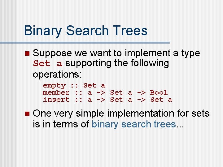
Binary Search Trees n Suppose we want to implement a type Set a supporting the following operations: empty : : Set a member : : a -> Set a -> Bool insert : : a -> Set a n One very simplementation for sets is in terms of binary search trees. . .

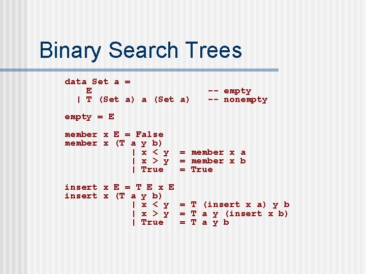
Binary Search Trees data Set a = E | T (Set a) a (Set a) -- empty -- nonempty = E member x E = False member x (T a y b) | x < y | x > y | True = member x a = member x b = True insert x E = T E x E insert x (T a y b) | x < y = T (insert x a) y b | x > y = T a y (insert x b) | True = T a y b

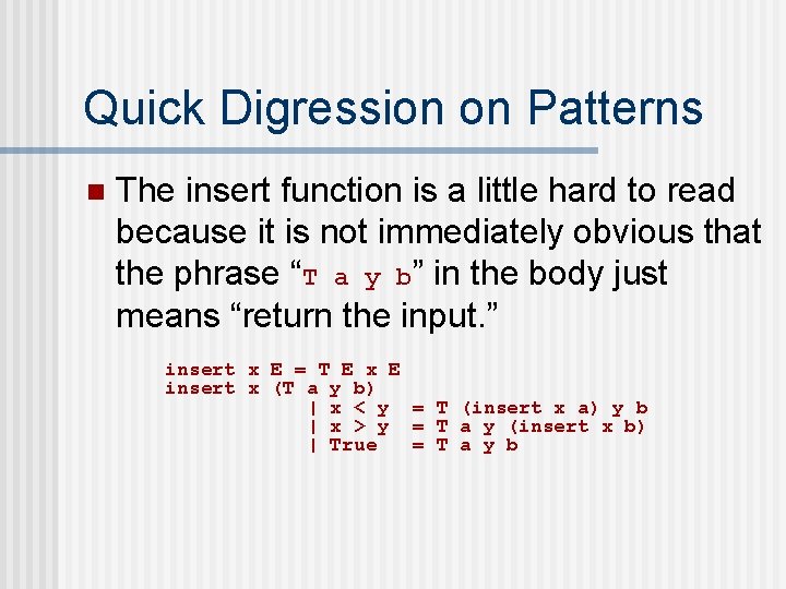
Quick Digression on Patterns n The insert function is a little hard to read because it is not immediately obvious that the phrase “T a y b” in the body just means “return the input. ” insert x E = T E x E insert x (T a y b) | x < y = T (insert x a) y b | x > y = T a y (insert x b) | True = T a y b

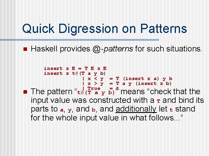
Quick Digression on Patterns n n Haskell provides @-patterns for such situations. insert x E = T E x E insert x t@(T a y b) | x < y = T (insert x a) y b | x > y = T a y (insert x b) | True = t The pattern “t@(T a y b)” means “check that the input value was constructed with a T and bind its parts to a, y, and b, and additionally let t stand for the whole input value in what follows. . . ”

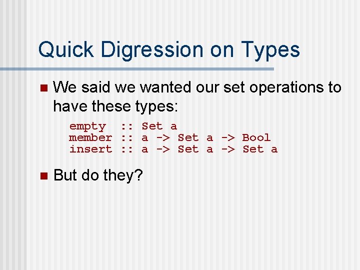
Quick Digression on Types n We said we wanted our set operations to have these types: empty : : Set a member : : a -> Set a -> Bool insert : : a -> Set a n But do they?

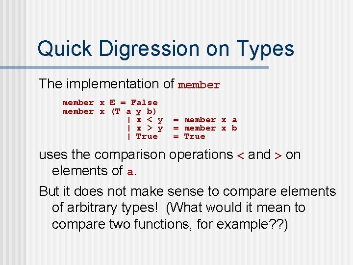
Quick Digression on Types The implementation of member x E = False member x (T a y b) | x < y | x > y | True = member x a = member x b = True uses the comparison operations < and > on elements of a. But it does not make sense to compare elements of arbitrary types! (What would it mean to compare two functions, for example? ? )

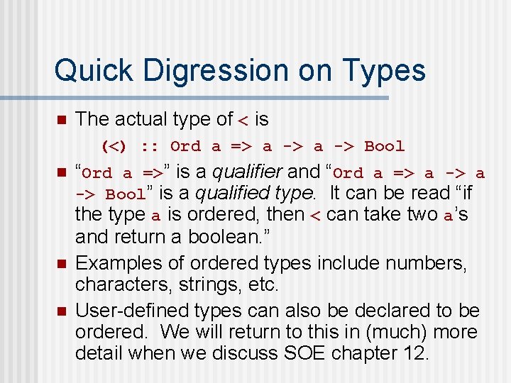
Quick Digression on Types n The actual type of < is (<) : : Ord a => a -> Bool n “Ord a =>” n n is a qualifier and “Ord a => a -> Bool” is a qualified type. It can be read “if the type a is ordered, then < can take two a’s and return a boolean. ” Examples of ordered types include numbers, characters, strings, etc. User-defined types can also be declared to be ordered. We will return to this in (much) more detail when we discuss SOE chapter 12.

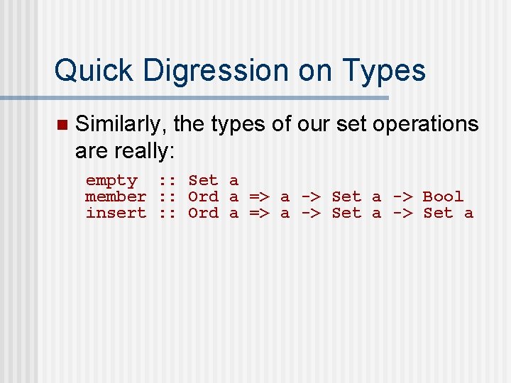
Quick Digression on Types n Similarly, the types of our set operations are really: empty : : Set a member : : Ord a => a -> Set a -> Bool insert : : Ord a => a -> Set a

Quick Digression on Types (end of digressions)

Balanced Trees n n n If our sets grow large, we may find that the simple binary tree implementation is not fast enough: in the worse case, each insert or member operation may take O(n) time! We can do much better by keeping the trees balanced. There are many ways of doing this. Let’s look at one fairly simple (but still very fast) one that you have probably seen before in an imperative setting: red-black trees.

Red-Black Trees n A red-black tree is a binary search tree where every node is additionally marked with a color (red or black) and in which the following invariants are maintained. . .

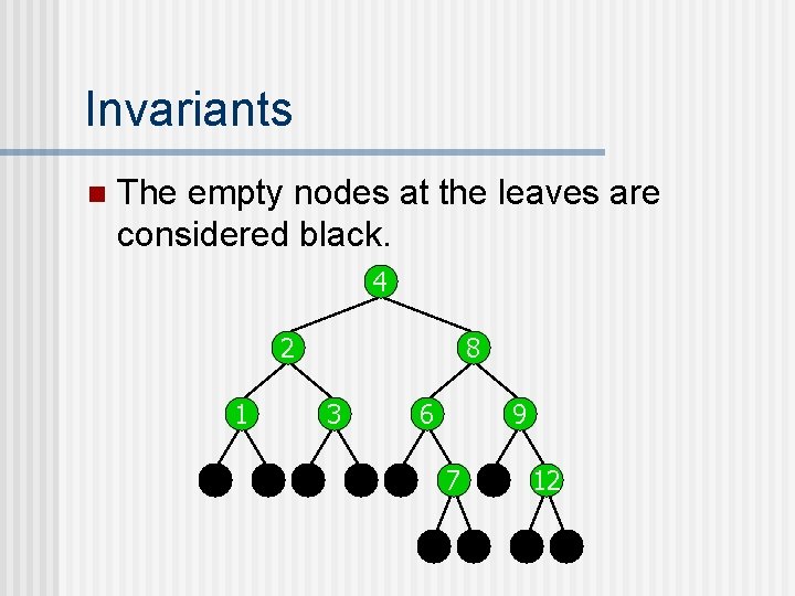
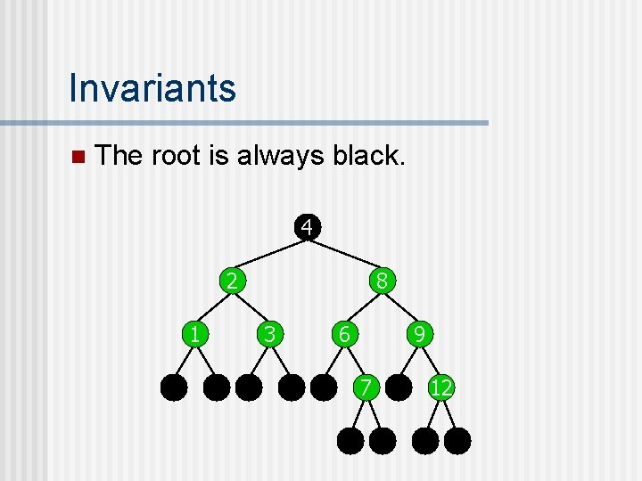
Invariants n The empty nodes at the leaves are considered black. 4 2 1 8 3 6 9 7 12

Invariants n The root is always black. 4 2 1 8 3 6 9 7 12

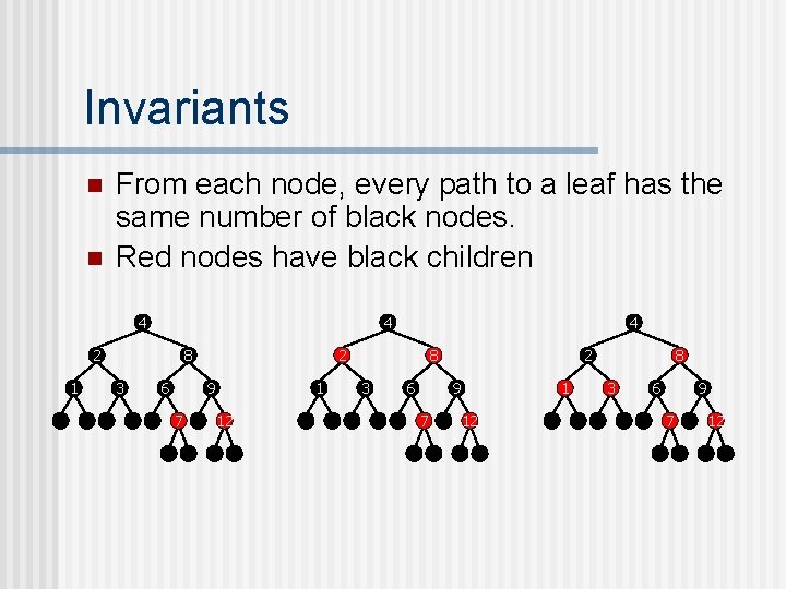
Invariants n n From each node, every path to a leaf has the same number of black nodes. Red nodes have black children 4 4 2 1 8 3 6 2 9 7 4 1 12 8 3 6 2 9 7 1 12 8 3 6 9 7 12

Invariants n n Together, these invariants imply that every redblack tree is “approximately balanced, ” in the sense that the longest path to an empty node is no more than twice the length of the shortest. From this, it follows that all operations will run in O(log 2 n) time. Now let’s look at the details. . .

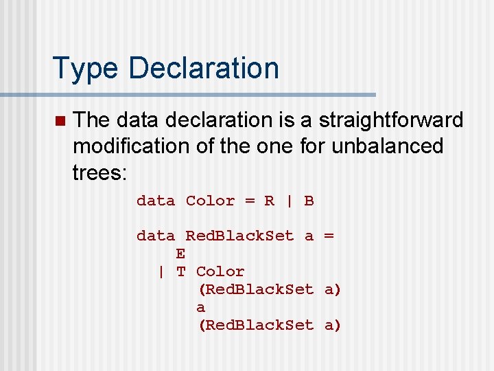
Type Declaration n The data declaration is a straightforward modification of the one for unbalanced trees: data Color = R | B data Red. Black. Set a = E | T Color (Red. Black. Set a) a (Red. Black. Set a)

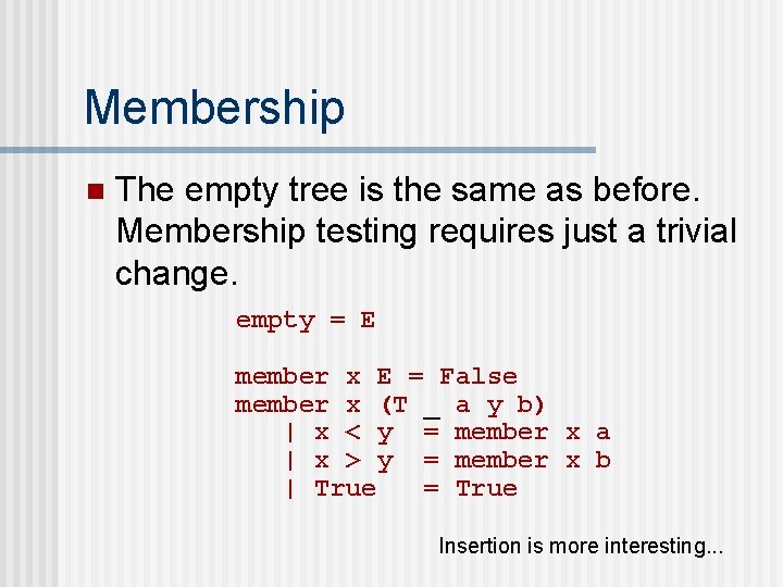
Membership n The empty tree is the same as before. Membership testing requires just a trivial change. empty = E member x E = False member x (T _ a y b) | x < y = member x a | x > y = member x b | True = True Insertion is more interesting. . .

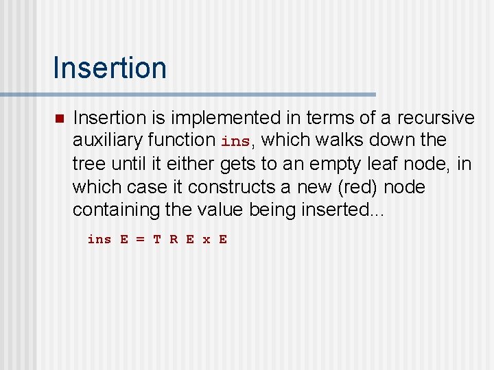
Insertion n Insertion is implemented in terms of a recursive auxiliary function ins, which walks down the tree until it either gets to an empty leaf node, in which case it constructs a new (red) node containing the value being inserted. . . ins E = T R E x E

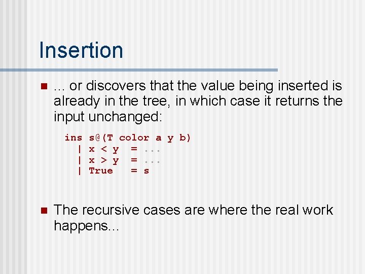
Insertion n . . . or discovers that the value being inserted is already in the tree, in which case it returns the input unchanged: ins | | | n s@(T color a y b) x < y =. . . x > y =. . . True = s The recursive cases are where the real work happens. . .

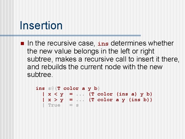
Insertion n In the recursive case, ins determines whether the new value belongs in the left or right subtree, makes a recursive call to insert it there, and rebuilds the current node with the new subtree. ins | | | s@(T color a y b) x < y =. . . (T color (ins a) y b) x > y =. . . (T color a y (ins b)) True = s

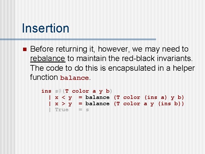
Insertion n Before returning it, however, we may need to rebalance to maintain the red-black invariants. The code to do this is encapsulated in a helper function balance. ins | | | s@(T color a y b) x < y = balance (T color (ins a) y b) x > y = balance (T color a y (ins b)) True = s

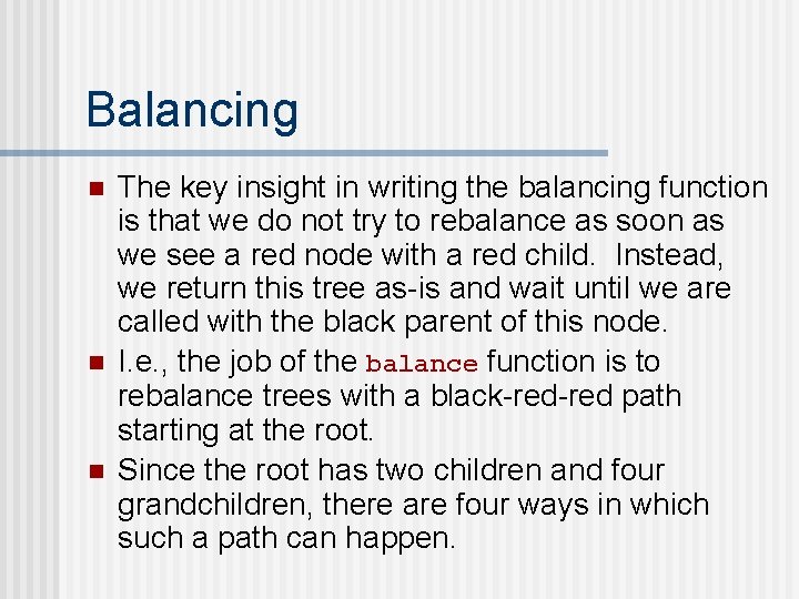
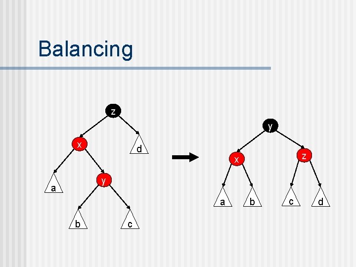
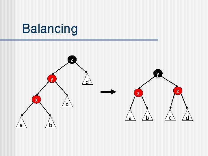
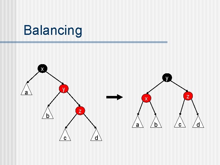
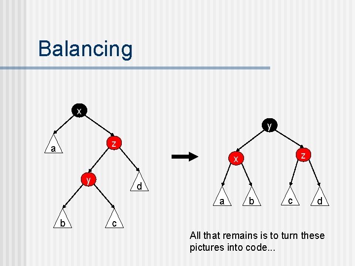
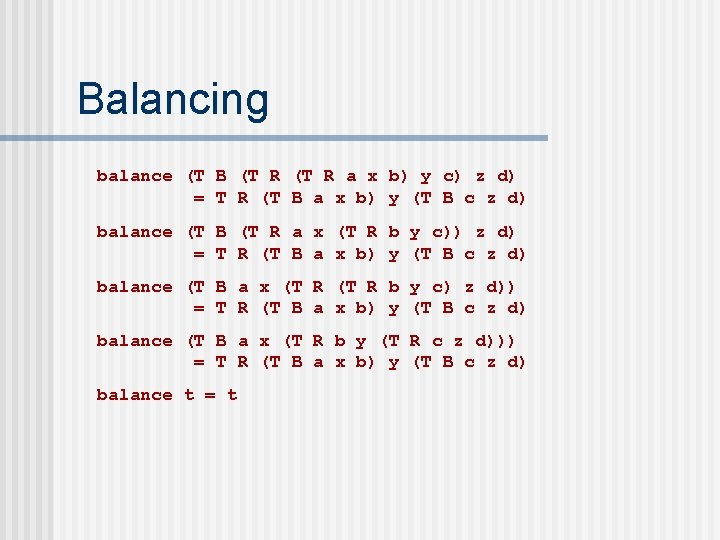
Balancing n n n The key insight in writing the balancing function is that we do not try to rebalance as soon as we see a red node with a red child. Instead, we return this tree as-is and wait until we are called with the black parent of this node. I. e. , the job of the balance function is to rebalance trees with a black-red path starting at the root. Since the root has two children and four grandchildren, there are four ways in which such a path can happen.

Balancing z y x d z x y a a b c d

Balancing z y y d x c a a z x b b c d

Balancing x y y a z x z b a c d b c d

Balancing x y z a z x y d a b b c d c All that remains is to turn these pictures into code. . .

Balancing balance (T B (T R a x b) y c) z d) = T R (T B a x b) y (T B c z d) balance (T B (T R a x (T R b y c)) z d) = T R (T B a x b) y (T B c z d) balance (T B a x (T R b y c) z d)) = T R (T B a x b) y (T B c z d) balance (T B a x (T R b y (T R c z d))) = T R (T B a x b) y (T B c z d) balance t = t

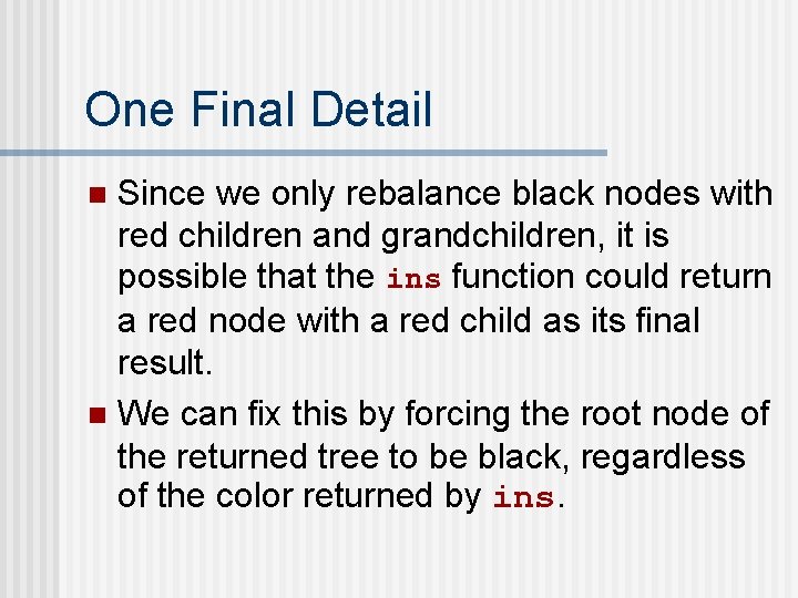
One Final Detail Since we only rebalance black nodes with red children and grandchildren, it is possible that the ins function could return a red node with a red child as its final result. n We can fix this by forcing the root node of the returned tree to be black, regardless of the color returned by ins. n

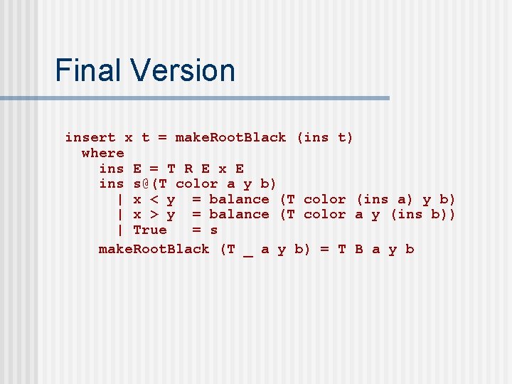
Final Version insert x t = make. Root. Black (ins t) where ins E = T R E x E ins s@(T color a y b) | x < y = balance (T color (ins a) y b) | x > y = balance (T color a y (ins b)) | True = s make. Root. Black (T _ a y b) = T B a y b

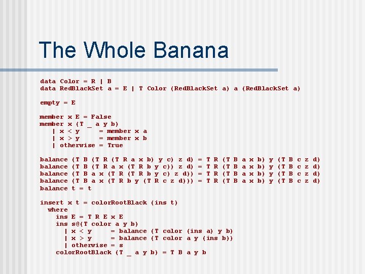
The Whole Banana data Color = R | B data Red. Black. Set a = E | T Color (Red. Black. Set a) a (Red. Black. Set a) empty = E member x E = False member x (T _ a y b) | x < y = member x a | x > y = member x b | otherwise = True balance balance (T B (T R a x b) y c) z d) (T B (T R a x (T R b y c)) z d) (T B a x (T R b y c) z d)) (T B a x (T R b y (T R c z d))) t = t insert x t = color. Root. Black where ins E = T R E x E ins s@(T color a y b) | x < y = balance | x > y = balance | otherwise = s color. Root. Black (T _ a y = = T T R R (T (T (ins t) (T color (ins a) y b) (T color a y (ins b)) b) = T B a y b B B a a x x b) b) y y (T (T B B c c z z d) d)

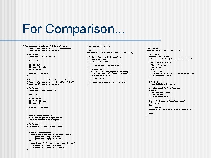
For Comparison. . . /* This function can be called only if K 2 has a left child */ /* Perform a rotate between a node (K 2) and its left child */ /* Update heights, then return new root */ static Position Single. Rotate. With. Left( Position K 2 ) { Position K 1; static Position X, P, GGP; static void Handle. Reorient( Element. Type Item, Red. Black. Tree T ) { X->Color = Red; /* Do the color flip */ X->Left->Color = Black; X->Right->Color = Black; K 1 = K 2 ->Left; K 2 ->Left = K 1 ->Right; K 1 ->Right = K 2; if( P->Color == Red ) /* Have to rotate */ { GP->Color = Red; if( (Item < GP->Element) != (Item < P->Element) ) P = Rotate( Item, GP ); /* Start double rotate */ X = Rotate( Item, GGP ); X->Color = Black; } T->Right->Color = Black; /* Make root black */ return K 1; /* New root */ } /* This function can be called only if K 1 has a right child */ /* Perform a rotate between a node (K 1) and its right child */ /* Update heights, then return new root */ Red. Black. Tree Insert( Element. Type Item, Red. Black. Tree T ) { X = P = GP = T; Null. Node->Element = Item; while( X->Element != Item ) /* Descend down the tree */ { GGP = GP; GP = P; P = X; if( Item < X->Element ) X = X->Left; else X = X->Right; if( X->Left->Color == Red && X->Right->Color == Red ) Handle. Reorient( Item, T ); } if( X != Null. Node ) return Null. Node; /* Duplicate */ } static Position Single. Rotate. With. Right( Position K 1 ) { Position K 2; X = malloc( sizeof( struct Red. Black. Node ) ); if( X == NULL ) Fatal. Error( "Out of space!!!" ); X->Element = Item; X->Left = X->Right = Null. Node; K 2 = K 1 ->Right; K 1 ->Right = K 2 ->Left; K 2 ->Left = K 1; if( Item < P->Element ) /* Attach to its parent */ P->Left = X; else P->Right = X; Handle. Reorient( Item, T ); /* Color it red; maybe rotate */ return K 2; /* New root */ } return T; /* Perform a rotation at node X */ /* (whose parent is passed as a parameter) */ /* The child is deduced by examining Item */ static Position Rotate( Element. Type Item, Position Parent ) { if( Item < Parent->Element ) return Parent->Left = Item < Parent->Left->Element ? Single. Rotate. With. Left( Parent->Left ) : Single. Rotate. With. Right( Parent->Left ); else return Parent->Right = Item < Parent->Right->Element ? Single. Rotate. With. Left( Parent->Right ) : Single. Rotate. With. Right( Parent->Right ); } }