Advanced Mathematics Advanced Mathematics Curve Fitting Interpolation and

Advanced Mathematics

Advanced Mathematics – Curve Fitting

Interpolation and Extrapolation In many cases, estimating values other than at the sampled data points is desired. For example, we might want to estimate what the temperature was at Temperatures 2: 30 pm or at 1: 00 pm. Interpolation means estimating the values in between recorded data points. Extrapolation is estimating outside of the bounds of the recorded data. One way to do this is to fit a curve to the data and use this for the estimations. Curve fitting is finding the curve that “best fits” the data. `

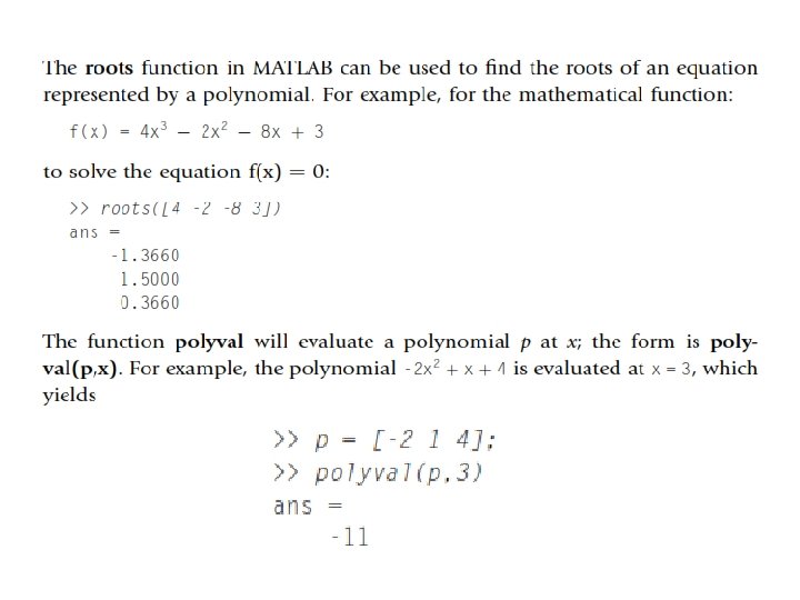
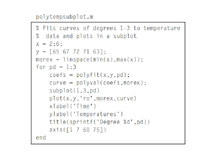
MATLAB has a function to do this called polyfit. The function polyfit finds the coefficients of the polynomial of the specified degree that best fits the data using a least squares algorithm. There are three arguments passed to the function: the vectors that represent the data and the degree of the desired polynomial. For example, to fit a straight line (degree 1) through the points representing temperatures, the call to the polyfit function would be

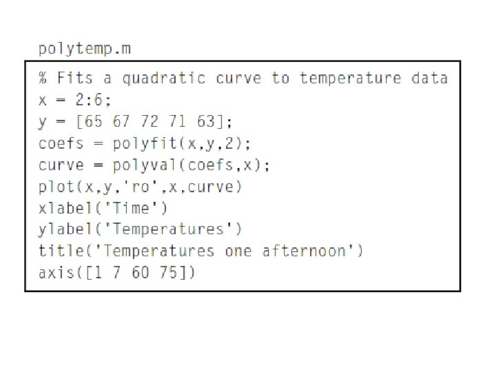
However, from the plot, it looks like a quadratic would be a much better fit. The following would create the vectors and then fit a polynomial of degree 2 through the data points, storing the values in a vector called coefs.

The function polyval can then be used to evaluate the polynomial at specified values. This results in y values for each point in the x vector, and stores them in a vector called curve.

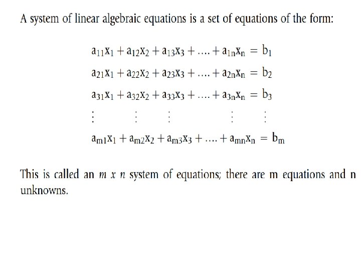
MATRIX SOLUTIONS TO SYSTEMS OF LINEAR ALGEBRAIC EQUATIONS • A linear algebraic equation is an equation of the form a 1 x 1 + a 2 x 2 + a 3 x 3 + … + an xn = b In the MATLAB product, to solve systems of equations, there are basically two methods: • n using a matrix representation • n using the solve function (which is part of Symbolic Math Toolbox).

Diagonal Matrices MATLAB has a function diag that will return the diagonal of a matrix as a column vector; transposing will result in a row vector instead.

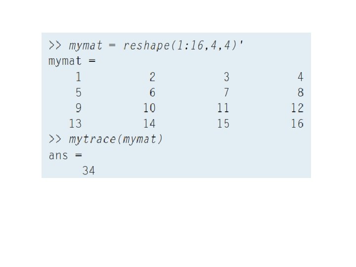
The diag function can also be used to take a vector of length n and create an n x n square diagonal matrix with the values from the vector on the diagonal: The trace of a square matrix is the sum of all of the elements on the diagonal.

>> trace (mymat)

• Identity matrix - >>eye(5) • lower triangular matrix – >>tril(mymat) • Upper triangular matrix – >>triu(mymat) MATLAB has functions triu and tril that will take a matrix and make it into an upper triangular or lower triangular matrix by replacing the appropriate elements with 0 s.

Matrix Operations • Transpose of a matrix – • Inverse of a matrix: MATLAB, has a function inv to compute a matrix inverse.

• Matrix augmentation means adding column(s) to the original matrix • In MATLAB, matrix augmentation can be accomplished using square brackets to concatenate the two matrices.

A solution set is the set of all possible solutions to the system of equations (all sets of values for the unknowns that satisfy the equations). All systems of linear equations have either: • no solutions • one solution • infinitely many solutions.

• The solution is then x = A-1 b. In MATLAB there are two simple ways to solve this. The built-in function inv can be used to get the inverse of A and then we multiply this by b, or we can use the divided into operator.

Determinant of a matrix

Symbolic Variables and Expressions MATLAB has a type called sym for symbolic variables and expressions; these work with strings. Symbolic variables can also store expressions.

All basic mathematical operations can be performed on symbolic variables and expressions (e. g. , add, subtract, multiply, divide, raise to a power, etc. ).

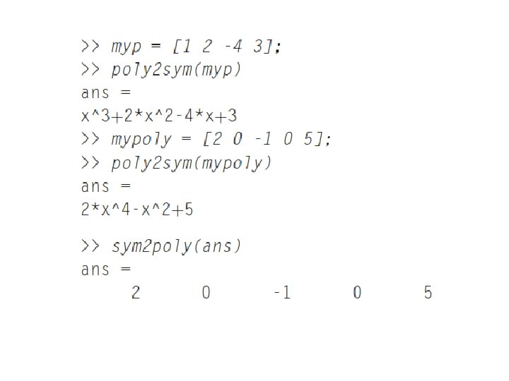
If using multiple variables as symbolic variable names is desired, the syms function is a shortcut instead of using sym repeatedly. >> syms x y z The built-in functions sym 2 poly and poly 2 sym convert from symbolic expressions to polynomial vectors and vice versa.

Simplification Functions There are several functions that work with symbolic expressions and simplify the terms. Not all expressions can be simplified, but the simplify function does whatever it can to simplify expressions, including gathering like terms.

The functions collect, expand, and factor work with polynomial expressions. The collect function collects coefficients. The expand function will multiply out terms, and factor will do the reverse:

The subs function will substitute a value for a symbolic variable in an expression.

Displaying Expressions There are several plot functions in MATLAB with names beginning with “ez” that perform the necessary conversions from symbolic expressions to numbers and plot them.

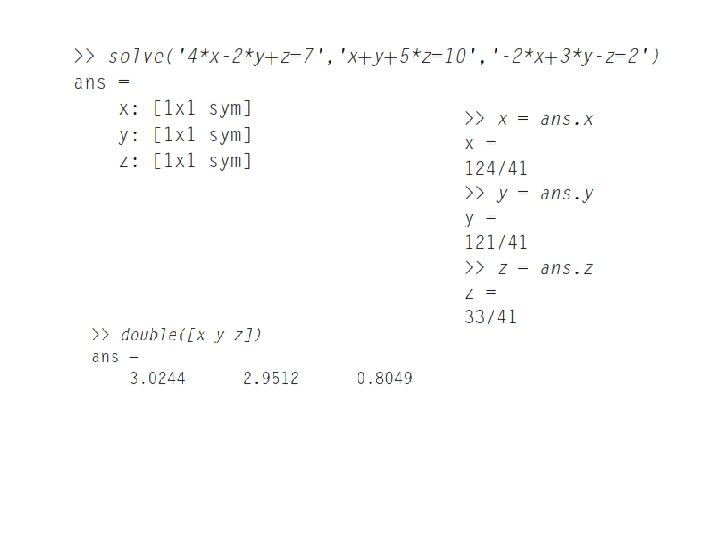
Solving Equations • The function solves an equation and returns the solution(s) as symbolic expressions. • If an expression is passed to the solve function rather than an equation, the solve function will set the expression equal to 0 and solve the resulting equation. • MATLAB can also solve sets of equations.

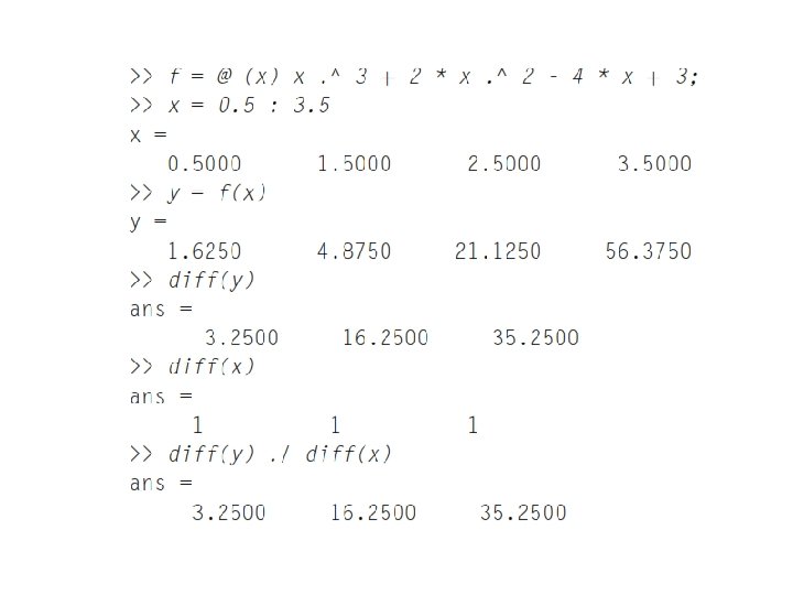
CALCULUS: INTEGRATION AND DIFFERENTIATION MATLAB has functions that perform common calculus operations on a mathematical function f(x), such as integration and differentiation

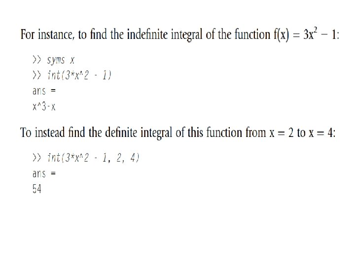
Integration and the Trapezoidal Rule The integral of a function f(x) between the limits given by x = a and x = b is written as and is defined as the area under the curve f(x) from a to b, as long as the function is above the x-axis. Numerical integration techniques involve approximating this.

for the function f(x) = 3 x 2 - 1

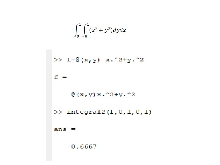
Other methods involve higher-order polynomials. The built-in function quad uses Simpson’s method. Three arguments are normally passed to it: the handle of the function, and the limits a and b.

• Differentiation

• The function polyval can then be used to find the derivative for certain values of x, such as for x = 1, 2 and 3:

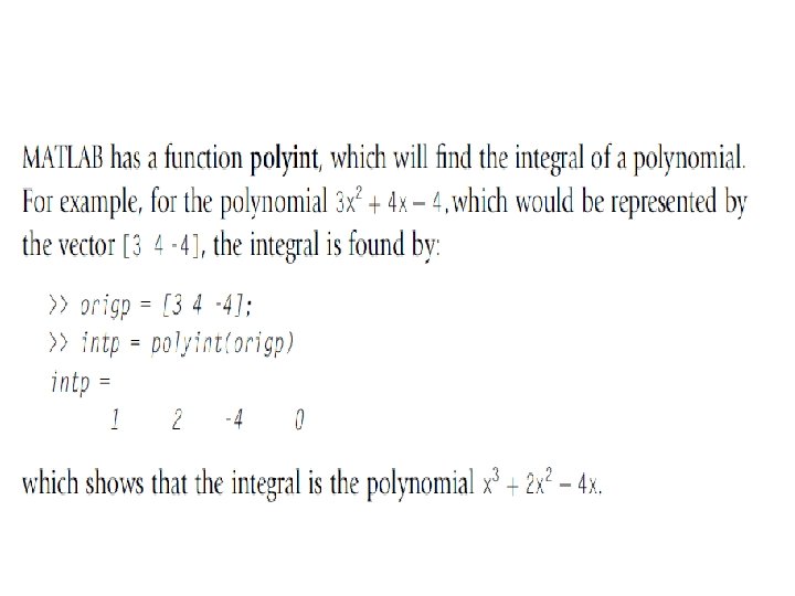
Calculus in Symbolic Math Toolbox There are several functions in Symbolic Math Toolbox to perform calculus operations symbolically (e. g. , diff to differentiate and int to integrate).

• Limits can be found using the limit function.

The syntax for second derivatives is >> diff (f, 2) The syntax for nth derivative is >> diff (f, n) The command diff can also compute partial derivatives of expressions involving several variables, as in diff(x^2*y, y), but to do multiple partials with respect to mixed variables you must use diff repeatedly, as in diff(sin (x*y/z), x), y)). (remember to declare y and z to be symbolic. )