Advanced Computer Vision Module 5 F 16 Carsten

![Structured Output Ad hoc definition (from [Nowozin et al. 2011]) Data that consists of Structured Output Ad hoc definition (from [Nowozin et al. 2011]) Data that consists of](https://slidetodoc.com/presentation_image_h2/ff193f6f98ccdf4f37d613b4e7fb9a64/image-24.jpg)

![Segmentation [Boykov& Jolly ICCV ‘ 01] E(x) = ∑ Fp xp+ Bp (1 -xp) Segmentation [Boykov& Jolly ICCV ‘ 01] E(x) = ∑ Fp xp+ Bp (1 -xp)](https://slidetodoc.com/presentation_image_h2/ff193f6f98ccdf4f37d613b4e7fb9a64/image-58.jpg)
![Grab. Cut [Rother, Kolmogorov, Blake, Siggraph ‘ 04] Fp(θF)xp+ Bp(θB)(1 -xp) + pq∑Є wpq|xp-xq| Grab. Cut [Rother, Kolmogorov, Blake, Siggraph ‘ 04] Fp(θF)xp+ Bp(θB)(1 -xp) + pq∑Є wpq|xp-xq|](https://slidetodoc.com/presentation_image_h2/ff193f6f98ccdf4f37d613b4e7fb9a64/image-60.jpg)
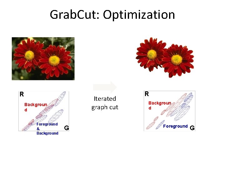
![Grab. Cut: Optimization [Rother, Kolmogorov, Blake, Siggraph ‘ 04] Image z and user input Grab. Cut: Optimization [Rother, Kolmogorov, Blake, Siggraph ‘ 04] Image z and user input](https://slidetodoc.com/presentation_image_h2/ff193f6f98ccdf4f37d613b4e7fb9a64/image-61.jpg)
- Slides: 64

Advanced Computer Vision (Module 5 F 16) Carsten Rother Pushmeet Kohli

Syllabus (updated) • L 1&2: Intro – Intro: Probabilistic models – Different approaches for learning – Generative/discriminative models, discriminative functions • L 3&4: Labelling Problems in Computer Vision – Graphical models – Expressing vision problems as labelling problems • L 5&6: Optimization - Message Passing (BP, TRW) - Submodularity and Graph Cuts - Move Making algorithms (Expansion/Swap/Range/Fusion) - LP Relaxations - Dual Decomposition

Syllabus (updated) • L 7&8 (8. 2): Optimization and Learning - compare max-margin vs. maximum likelihood • L 9&10 (15. 2): Case Studies - tbd … Decision Trees and Random Fields, Kinect Person detection • L 11&12 (22. 2): Optimization Comparison, Case Studies (tbd)

Books 1. Advances in Markov Random Fields for Computer Vision. MIT Press 2011. (Edited by Andrew Blake, Pushmeet Kohli and Carsten Rother) 2. Pattern Recognition and Machine Learning, Springer 2006, by Chris Bishop 3. Structured Learning and Prediction in Computer Vision (Sebastian Nowozin and Christoph H. Lampert; Foundations and Trends in Computer Graphics and Vision series of now publishers, 2011). 4. Computer Vision, Springer 2010, by Rick Szeliski

A gentle Start: Interactive Image Segmentation and Probabilities

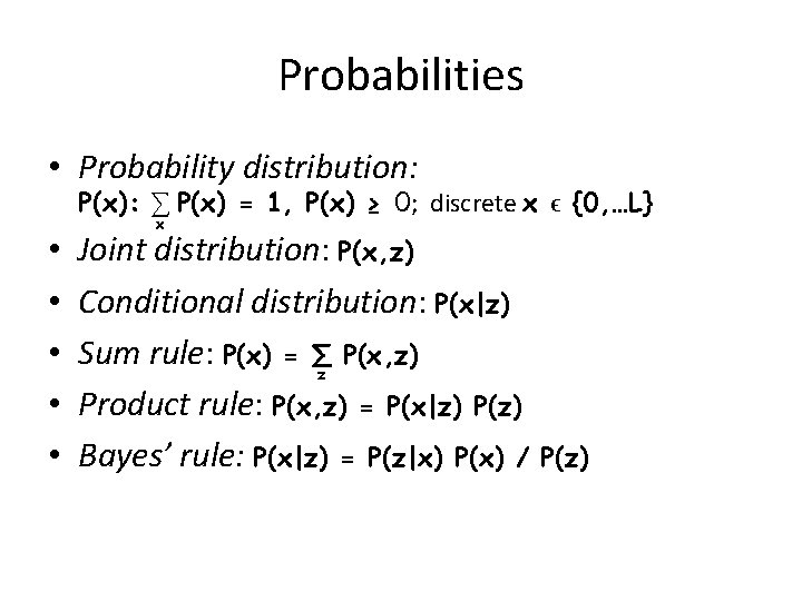
Probabilities • Probability distribution: P(x): ∑ P(x) = 1, P(x) ≥ 0; discrete x ϵ {0, …L} • • • x Joint distribution: P(x, z) Conditional distribution: P(x|z) Sum rule: P(x) = ∑z P(x, z) Product rule: P(x, z) = P(x|z) P(z) Bayes’ rule: P(x|z) = P(z|x) P(x) / P(z)

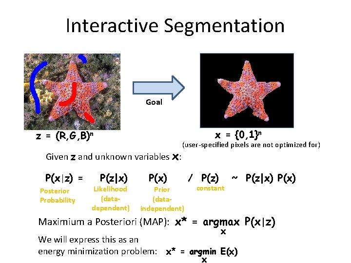
Interactive Segmentation Goal x = {0, 1}n z = (R, G, B)n Given z and unknown variables x: P(x|z) = Posterior Probability P(z|x) Likelihood (datadependent) (user-specified pixels are not optimized for) P(x) Prior (dataindependent) / P(z) constant ~ P(z|x) P(x) Maximium a Posteriori (MAP): x* = argmax P(x|z) x We will express this as an energy minimization problem: x* = argmin E(x) x

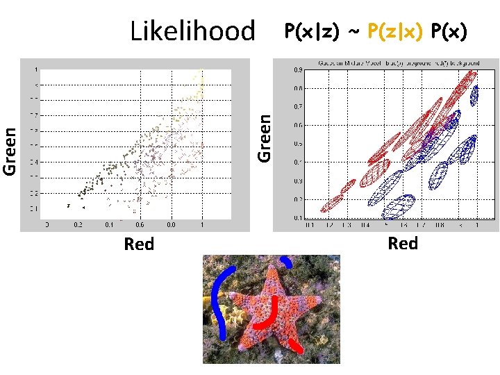
P(x|z) ~ P(z|x) P(x) Green Likelihood Red

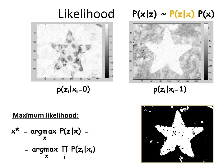
Likelihood p(zi|xi=0) Maximum likelihood: x* = argmax P(z|x) = x = argmax ∏ P(zi|xi) x i P(x|z) ~ P(z|x) P(x) p(zi|xi=1)

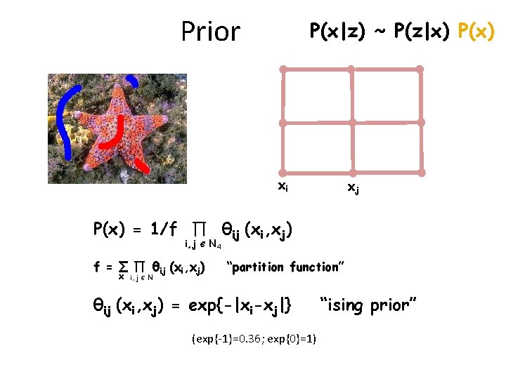
Prior P(x|z) ~ P(z|x) P(x) xi xj P(x) = 1/f ∏ θij (xi, xj) i, j Є f = ∑ ∏ θij (xi, xj) x i, j Є N N 4 “partition function” θij (xi, xj) = exp{-|xi-xj|} (exp{-1}=0. 36; exp{0}=1) “ising prior”

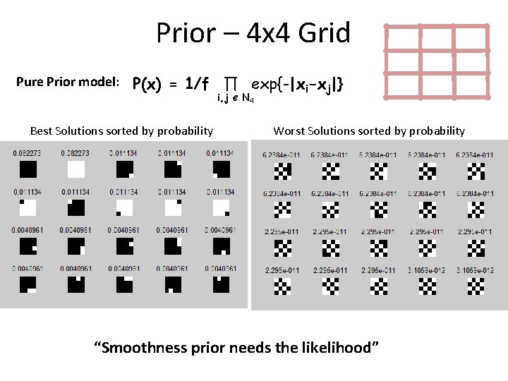
Prior – 4 x 4 Grid Pure Prior model: P(x) = 1/f ∏ exp{-|xi-xj|} i, j Best Solutions sorted by probability Є N 4 Worst Solutions sorted by probability “Smoothness prior needs the likelihood”

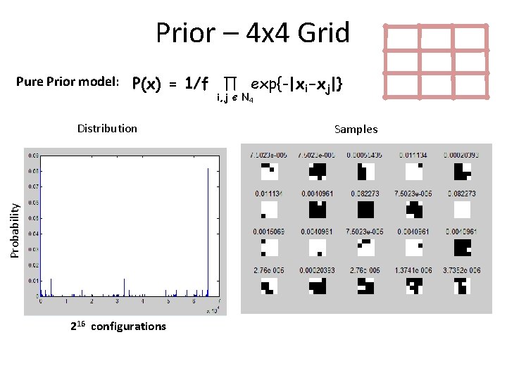
Prior – 4 x 4 Grid Pure Prior model: P(x) = 1/f ∏ exp{-|xi-xj|} i, j Probability Distribution 216 configurations Є N 4 Samples

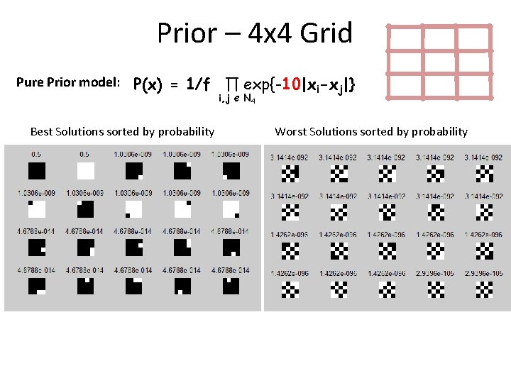
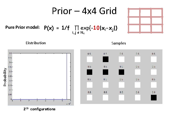
Prior – 4 x 4 Grid Pure Prior model: P(x) = 1/f ∏ exp{-10|xi-xj|} i, j Best Solutions sorted by probability Є N 4 Worst Solutions sorted by probability

Prior – 4 x 4 Grid Pure Prior model: P(x) = 1/f ∏ exp{-10|xi-xj|} i, j Probability Distribution 216 configurations Є N 4 Samples

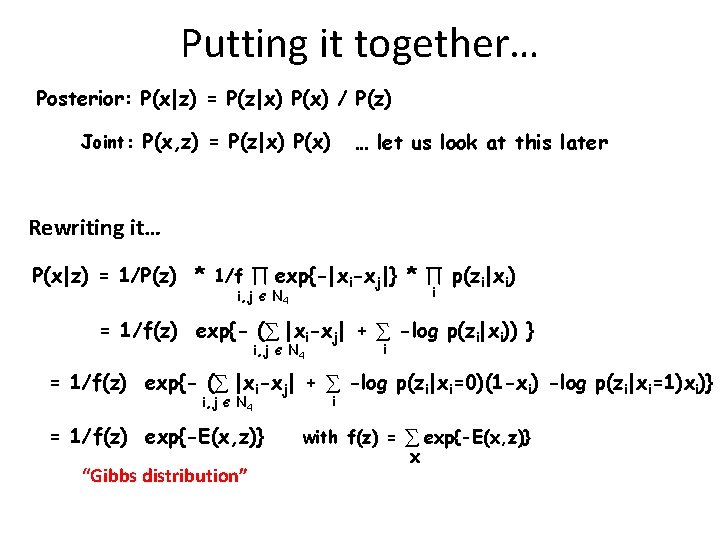
Putting it together… Posterior: P(x|z) = P(z|x) P(x) / P(z) Joint: P(x, z) = P(z|x) P(x) … let us look at this later Rewriting it… P(x|z) = 1/P(z) * 1/f ∏ exp{-|xi-xj|} * ∏ p(zi|xi) i, j Є i N 4 = 1/f(z) exp{- (∑ |xi-xj| + ∑ -log p(zi|xi)) } i, j Є i N 4 = 1/f(z) exp{- (∑ |xi-xj| + ∑ -log p(zi|xi=0)(1 -xi) -log p(zi|xi=1)xi)} i, j Є N 4 = 1/f(z) exp{-E(x, z)} “Gibbs distribution” i with f(z) = ∑ exp{-E(x, z)} x

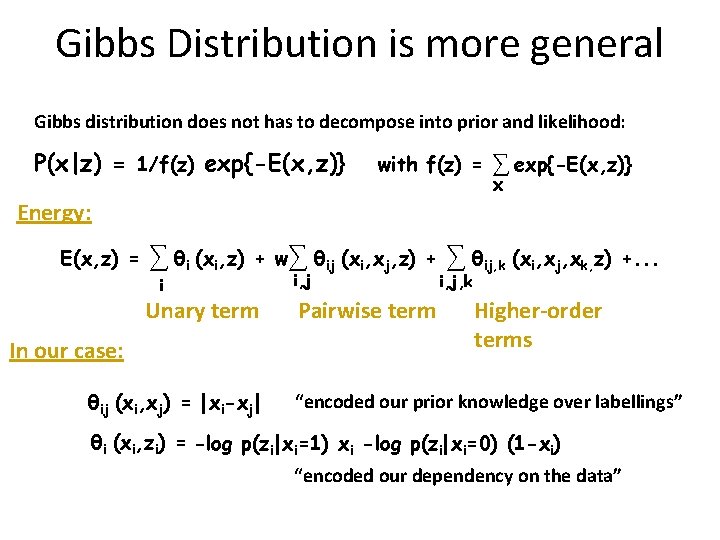
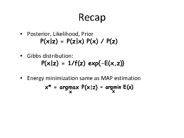
Gibbs Distribution is more general Gibbs distribution does not has to decompose into prior and likelihood: P(x|z) = 1/f(z) exp{-E(x, z)} with f(z) = ∑ exp{-E(x, z)} x Energy: E(x, z) = ∑ θi (xi, z) i + w∑ θij (xi, xj, z) + Unary term In our case: θij (xi, xj) = |xi-xj| i, j Pairwise term ∑ θij, k (xi, xj, xk, z) i, j, k +. . . Higher-order terms “encoded our prior knowledge over labellings” θi (xi, zi) = -log p(zi|xi=1) xi -log p(zi|xi=0) (1 -xi) “encoded our dependency on the data”

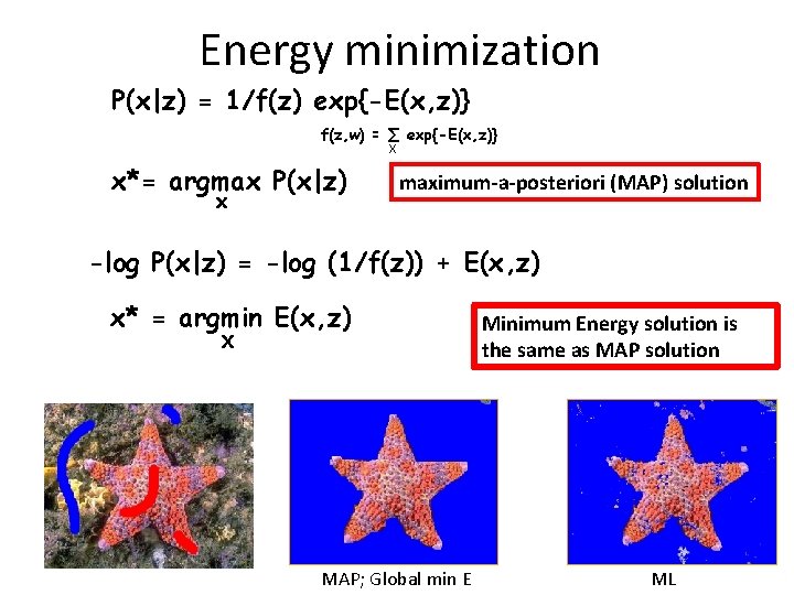
Energy minimization P(x|z) = 1/f(z) exp{-E(x, z)} f(z, w) = ∑ exp{-E(x, z)} X x*= argmax P(x|z) x maximum-a-posteriori (MAP) solution -log P(x|z) = -log (1/f(z)) + E(x, z) x* = argmin E(x, z) X MAP; Global min E Minimum Energy solution is the same as MAP solution ML

Recap • Posterior, Likelihood, Prior P(x|z) = P(z|x) P(x) / P(z) • Gibbs distribution: P(x|z) = 1/f(z) exp{-E(x, z)} • Energy minimization same as MAP estimation x* = argmax P(x|z) = argmin E(x) x x

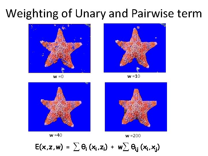
Weighting of Unary and Pairwise term w =0 w =10 w =40 w =200 E(x, z, w) = ∑ θi (xi, zi) + w∑ θij (xi, xj)

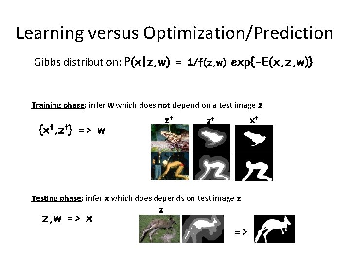
Learning versus Optimization/Prediction Gibbs distribution: P(x|z, w) = 1/f(z, w) exp{-E(x, z, w)} Training phase: infer w which does not depend on a test image z {xt, zt} => w zt xt zt Testing phase: infer x which does depends on test image z z z, w => x =>

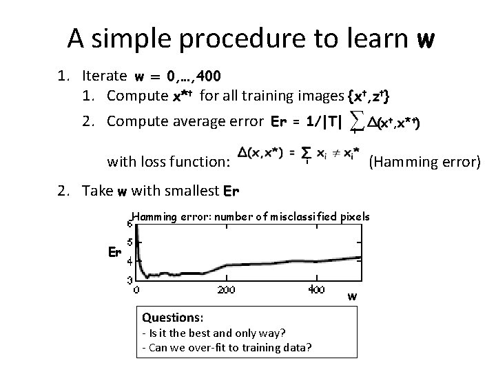
A simple procedure to learn w 1. Iterate w = 0, …, 400 1. Compute x*t for all training images {xt, zt} 2. Compute average error Er = 1/|T| with loss function: ∑ Δ(x , x* ) t t (Hamming error) i 2. Take w with smallest Er Hamming error: number of misclassified pixels Er w Questions: - Is it the best and only way? - Can we over-fit to training data? t

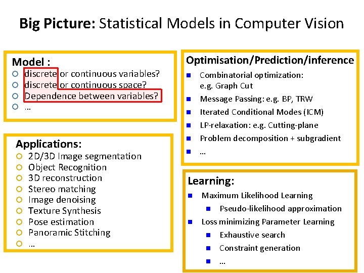
Big Picture: Statistical Models in Computer Vision Model : Optimisation/Prediction/inference n discrete or continuous variables? discrete or continuous space? Dependence between variables? … n n n Applications: 2 D/3 D Image segmentation Object Recognition 3 D reconstruction Stereo matching Image denoising Texture Synthesis Pose estimation Panoramic Stitching … n n Combinatorial optimization: e. g. Graph Cut Message Passing: e. g. BP, TRW Iterated Conditional Modes (ICM) LP-relaxation: e. g. Cutting-plane Problem decomposition + subgradient … Learning: n n Maximum Likelihood Learning n Pseudo-likelihood approximation Loss minimizing Parameter Learning n Exhaustive search n Constraint generation n …

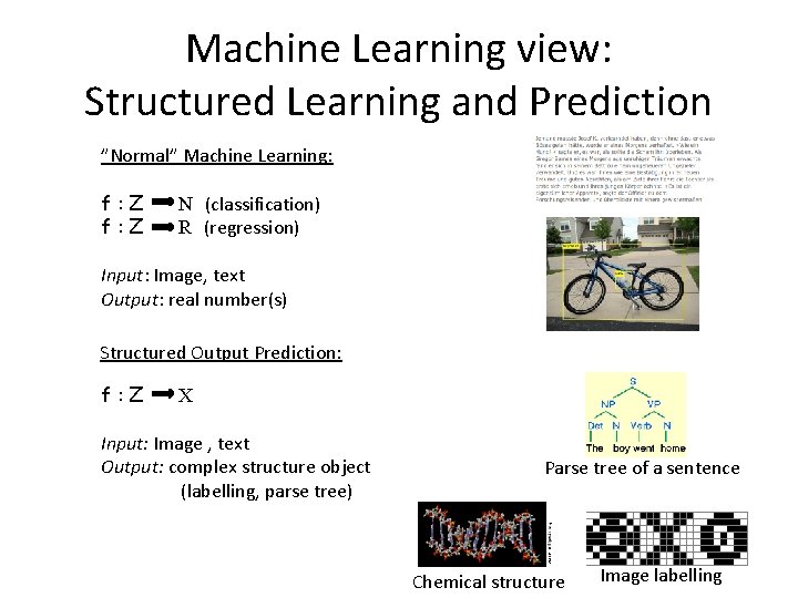
Machine Learning view: Structured Learning and Prediction ”Normal” Machine Learning: f: Z N (classification) R (regression) Input: Image, text Output: real number(s) Structured Output Prediction: f: Z X Input: Image , text Output: complex structure object (labelling, parse tree) Parse tree of a sentence Chemical structure Image labelling
![Structured Output Ad hoc definition from Nowozin et al 2011 Data that consists of Structured Output Ad hoc definition (from [Nowozin et al. 2011]) Data that consists of](https://slidetodoc.com/presentation_image_h2/ff193f6f98ccdf4f37d613b4e7fb9a64/image-24.jpg)
Structured Output Ad hoc definition (from [Nowozin et al. 2011]) Data that consists of several parts, and not only the parts themselves contain information, but also the way in which the parts belong together.

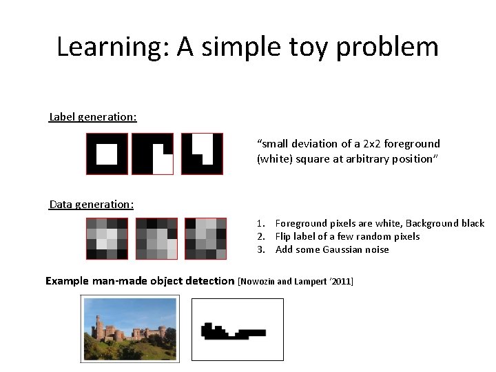
Learning: A simple toy problem Label generation: “small deviation of a 2 x 2 foreground (white) square at arbitrary position” Data generation: 1. Foreground pixels are white, Background black 2. Flip label of a few random pixels 3. Add some Gaussian noise Example man-made object detection [Nowozin and Lampert ‘ 2011]

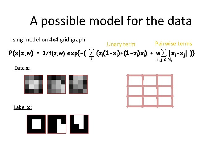
A possible model for the data Ising model on 4 x 4 grid graph: Pairwise terms Unary term P(x|z, w) = 1/f(z, w) exp{-( ∑ (zi(1 -xi)+(1 -zi)xi) + w∑ |xi-xj| )} i Data z: Label x: i, j Є N 4

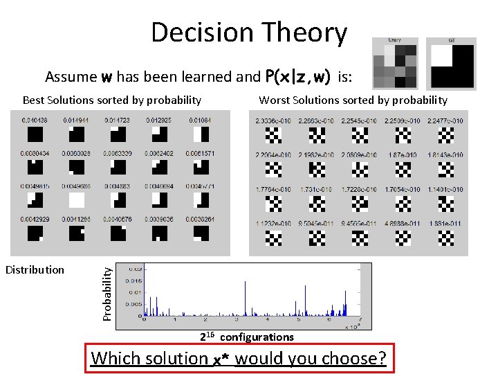
Decision Theory Assume w has been learned and P(x|z, w) is: Distribution Worst Solutions sorted by probability Probability Best Solutions sorted by probability 216 configurations Which solution x* would you choose?

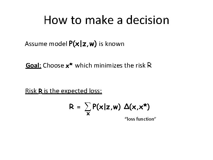
How to make a decision Assume model P(x|z, w) is known Goal: Choose x* which minimizes the risk R Risk R is the expected loss: R = ∑ P(x|z, w) x Δ(x, x*) “loss function”

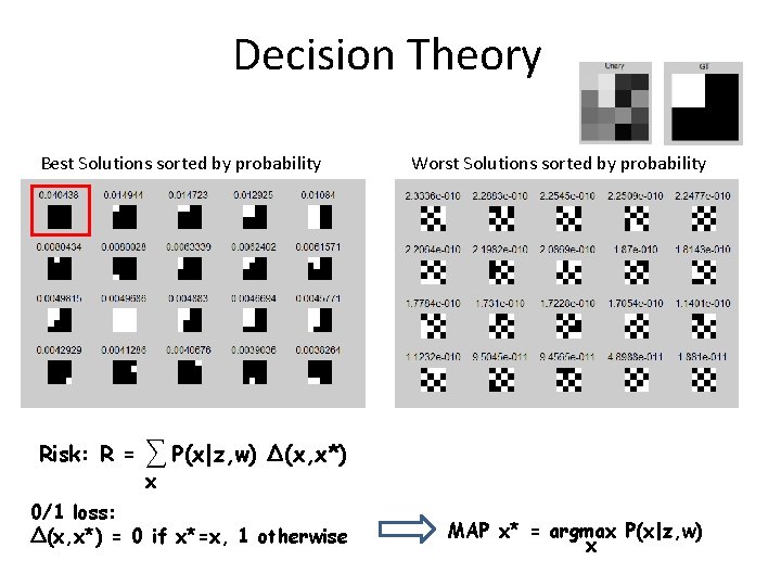
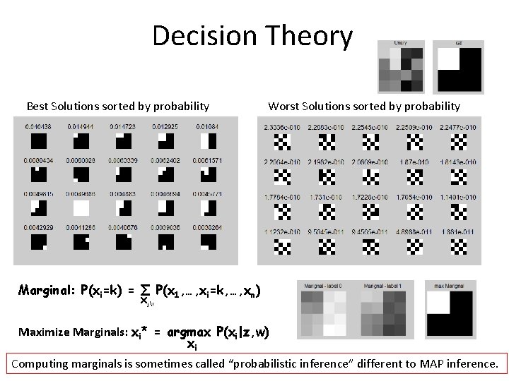
Decision Theory Best Solutions sorted by probability Risk: R = ∑ P(x|z, w) x Worst Solutions sorted by probability Δ(x, x*) 0/1 loss: Δ(x, x*) = 0 if x*=x, 1 otherwise MAP x* = argmax P(x|z, w) x

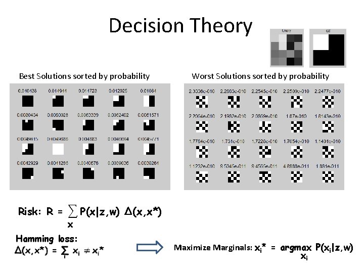
Decision Theory Best Solutions sorted by probability ∑ P(x|z, w) Risk: R = x Hamming loss: i Worst Solutions sorted by probability Δ(x, x*) Maximize Marginals: xi* = argmax P(xi|z, w) xi

Decision Theory Best Solutions sorted by probability Worst Solutions sorted by probability Marginal: P(xi=k) = ∑ P(x 1, …, xi=k, …, xn) Xji Maximize Marginals: xi* = argmax P(xi|z, w) xi Computing marginals is sometimes called “probabilistic inference” different to MAP inference.

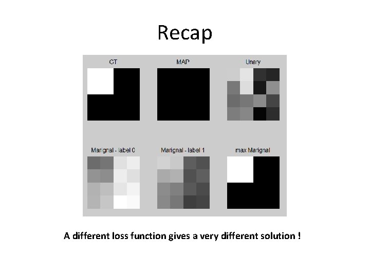
Recap A different loss function gives a very different solution !

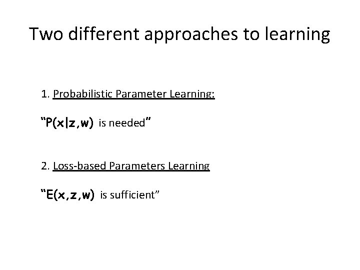
Two different approaches to learning 1. Probabilistic Parameter Learning: “P(x|z, w) is needed” 2. Loss-based Parameters Learning “E(x, z, w) is sufficient”

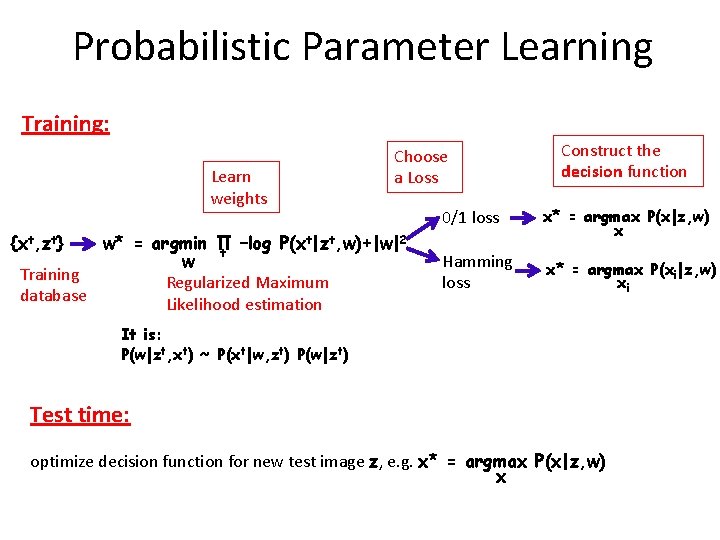
Probabilistic Parameter Learning Training: Learn weights {xt, zt} Choose a Loss t|zt, w)+|w|2 w* = argmin Π –log P(x t w Training Regularized Maximum database Likelihood estimation Construct the decision function 0/1 loss x* = argmax P(x|z, w) x Hamming loss x* = argmax P(xi|z, w) xi It is: P(w|zt, xt) ~ P(xt|w, zt) P(w|zt) Test time: optimize decision function for new test image z, e. g. x* = argmax P(x|z, w) x

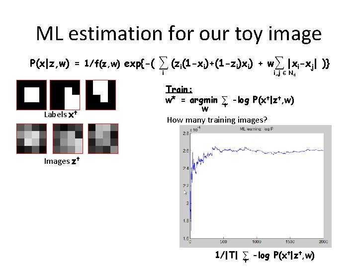
ML estimation for our toy image P(x|z, w) = 1/f(z, w) exp{-( Labels xt ∑ (zi(1 -xi)+(1 -zi)xi) i + w∑ |xi-xj| )} i, j Є N 4 Train: w* = argmin ∑ -log P(xt|zt, w) t w How many training images? PLOT Images zt 1/|T| ∑ -log P(xt|zt, w) t

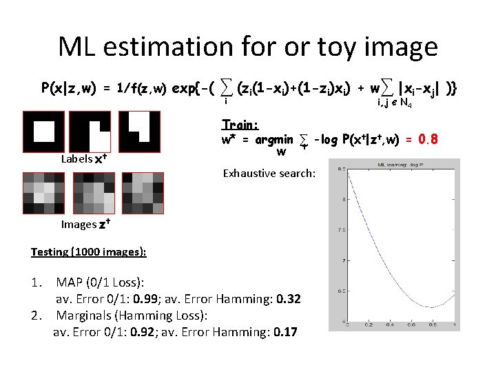
ML estimation for or toy image P(x|z, w) = 1/f(z, w) exp{-( Labels xt ∑ (zi(1 -xi)+(1 -zi)xi) i + w∑ |xi-xj| )} i, j Є N 4 Train: w* = argmin ∑ -log P(xt|zt, w) = 0. 8 w t Exhaustive search: Images zt Testing (1000 images): 1. MAP (0/1 Loss): av. Error 0/1: 0. 99; av. Error Hamming: 0. 32 2. Marginals (Hamming Loss): av. Error 0/1: 0. 92; av. Error Hamming: 0. 17

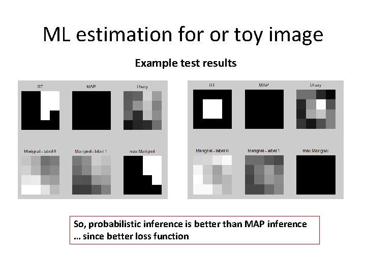
ML estimation for or toy image Example test results So, probabilistic inference is better than MAP inference … since better loss function

Two different approaches to learning 1. Probabilistic Parameter Learning: “P(x|z, w) is needed” 2. Loss-based Parameters Learning “E(x, z, w) is sufficient”

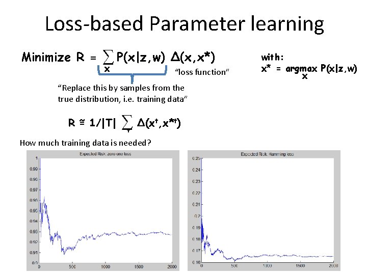
Loss-based Parameter learning Minimize R = ∑ P(x|z, w) x Δ(x, x*) “loss function” “Replace this by samples from the true distribution, i. e. training data” ~ 1/|T| R = ∑ Δ(xt, x*t) t How much training data is needed? with: x* = argmax P(x|z, w) x

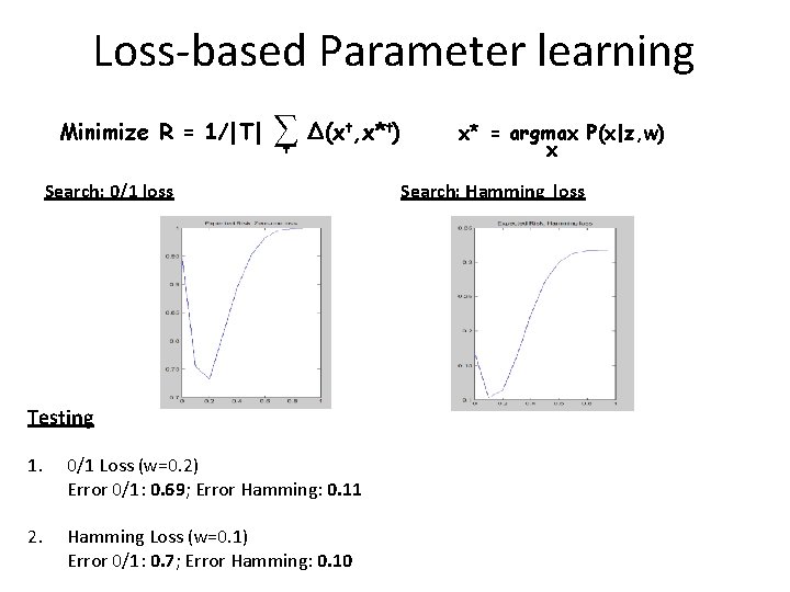
Loss-based Parameter learning Minimize R = 1/|T| ∑ Δ(xt, x*t) t Search: 0/1 loss Testing 1. 0/1 Loss (w=0. 2) Error 0/1: 0. 69; Error Hamming: 0. 11 2. Hamming Loss (w=0. 1) Error 0/1: 0. 7; Error Hamming: 0. 10 x* = argmax P(x|z, w) x Search: Hamming loss

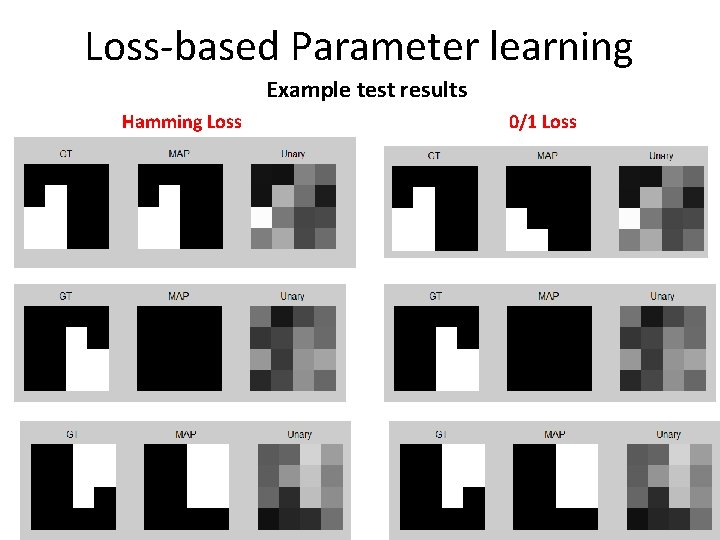
Loss-based Parameter learning Example test results Hamming Loss 0/1 Loss

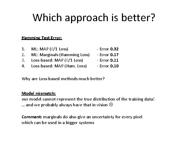
Which approach is better? Hamming Test Error: 1. 2. 3. 4. ML: MAP (0/1 Loss) ML: Marginals (Hamming Loss) Loss-based: MAP (0/1 Loss) Loss-based: MAP (Ham. Loss) - Error 0. 32 - Error 0. 17 - Error 0. 11 - Error 0. 10 Why are Loss-based methods much better? Model mismatch: our model cannot represent the true distribution of the training data! … and we probably always have that in vision Comment: marginals do also give an uncertainty for every pixel which can be used in a bigger systems

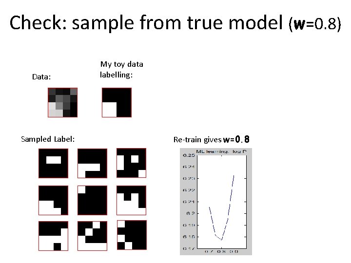
Check: sample from true model (w=0. 8) Data: Sampled Label: My toy data labelling: Re-train gives w=0. 8

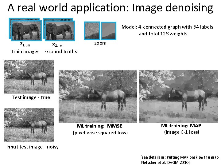
A real world application: Image denoising Model: 4 -connected graph with 64 labels and total 128 weights Train images zoom x 1. . m Z 1. . m Ground truths Test image - true ML training: MMSE (pixel-wise squared loss) ML training: MAP (image 0 -1 loss) Input test image - noisy [see details in: Putting MAP back on the map, Pletscher et al. DAGM 2010]

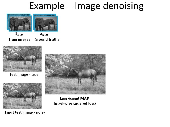
Example – Image denoising x 1. . m Z 1. . m Train images Ground truths Test image - true Loss-based MAP (pixel-wise squared loss) Input test image - noisy

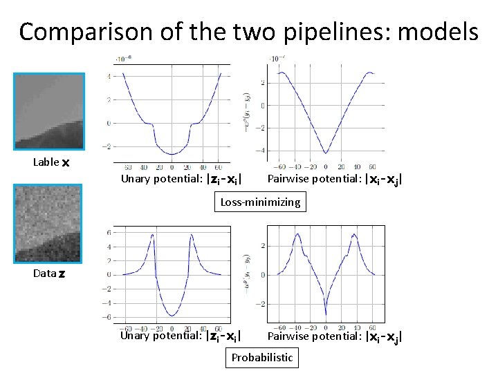
Comparison of the two pipelines: models Lable x Unary potential: |zi-xi| Pairwise potential: |xi-xj| Loss-minimizing Data z Unary potential: |zi-xi| Pairwise potential: |xi-xj| Probabilistic

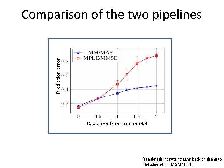
Prediction error Comparison of the two pipelines Deviation from true model [see details in: Putting MAP back on the map, Pletscher et al. DAGM 2010]

Recap • Loss functions • Two Pipelines for Parameter learning – Loss-based – Probabilistic • MAP inference is good, if trained well

Another Machine Learning view We can identify 3 different approaches: [see details in Bishop, page 42 ff]: • Generative (probabilistic) models • Discriminative functions

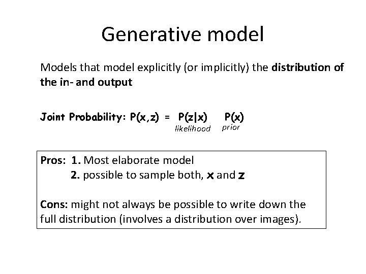
Generative model Models that model explicitly (or implicitly) the distribution of the in- and output Joint Probability: P(x, z) = P(z|x) likelihood P(x) prior Pros: 1. Most elaborate model 2. possible to sample both, x and z Cons: might not always be possible to write down the full distribution (involves a distribution over images).

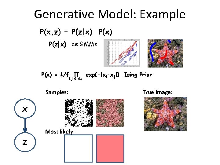
Generative Model: Example P(x, z) = P(z|x) as GMMs P(x) = 1/f ∏ i, j Є N 4 Samples: x z Most likely: exp{-|xi-xj|} Ising Prior True image:

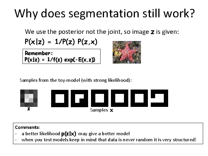
Why does segmentation still work? We use the posterior not the joint, so image z is given: P(x|z) = 1/P(z) P(z, x) Remember: P(x|z) = 1/f(z) exp{-E(x, z)} Samples from the toy-model (with strong likelihood): z Samples x Comments: - a better likelihood p(z|x) may give a better model - when you test models keep in mind that data is never random it is very structured!

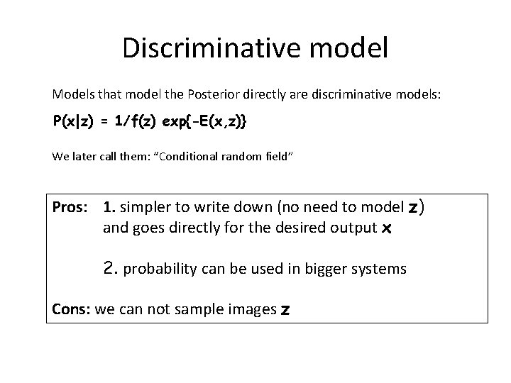
Discriminative model Models that model the Posterior directly are discriminative models: P(x|z) = 1/f(z) exp{-E(x, z)} We later call them: “Conditional random field” Pros: 1. simpler to write down (no need to model z) and goes directly for the desired output x 2. probability can be used in bigger systems Cons: we can not sample images z

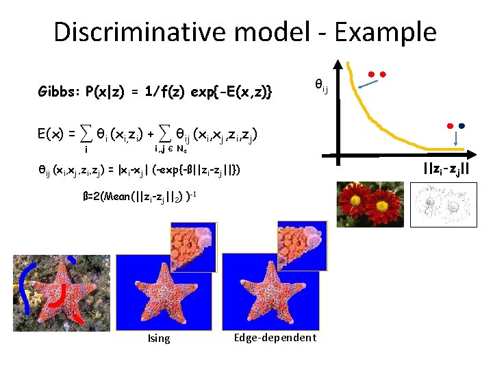
Discriminative model - Example Gibbs: P(x|z) = 1/f(z) exp{-E(x, z)} E(x) = θij ∑ θi (xi, zi) + ∑ θij (xi, xj, zi, zj) i i, j Є N 4 θij (xi, xj, zi, zj) = |xi-xj| (-exp{-ß||zi-zj||}) ß=2(Mean(||zi-zj||2) )-1 Ising Edge-dependent ||zi-zj||

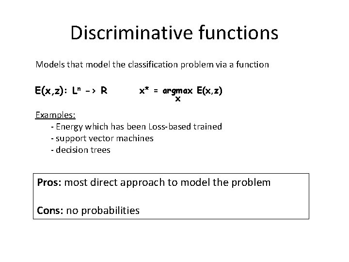
Discriminative functions Models that model the classification problem via a function E(x, z): Ln -> R x* = argmax E(x, z) x Examples: - Energy which has been Loss-based trained - support vector machines - decision trees Pros: most direct approach to model the problem Cons: no probabilities

Recap • Generative (probabilistic) models • Discriminative functions

Image segmentation … the full story … a meeting with the Queen
![Segmentation Boykov Jolly ICCV 01 Ex Fp xp Bp 1 xp Segmentation [Boykov& Jolly ICCV ‘ 01] E(x) = ∑ Fp xp+ Bp (1 -xp)](https://slidetodoc.com/presentation_image_h2/ff193f6f98ccdf4f37d613b4e7fb9a64/image-58.jpg)
Segmentation [Boykov& Jolly ICCV ‘ 01] E(x) = ∑ Fp xp+ Bp (1 -xp) + ∑ wpq|xp-xq| pϵV pq ϵ E F p = 0 Bp = ∞ F p = ∞ Bp = 0 wpq = wi + wc exp(-wβ||zp-zq||2) Graph Cut: Global optimum in polynomial time ~0. 3 sec for 1 MPixel image [Boykov, Kolmogorov, PAMI ‘ 04] Image z and user input Output x* = argmin E(x) ϵ {0, 1} x How to prevent the trivial solution?

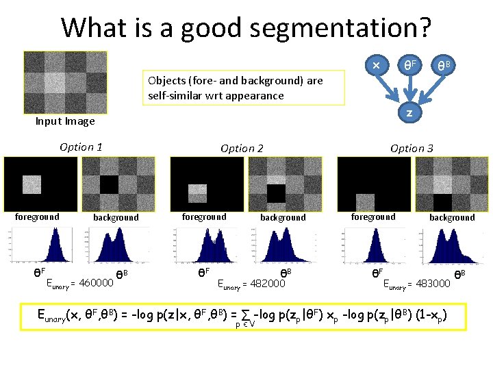
What is a good segmentation? x θF Objects (fore- and background) are self-similar wrt appearance z Input Image Option 1 foreground θF Option 2 background Eunary = 460000 θB θB foreground θF Option 3 background θB Eunary = 482000 foreground θF background Eunary = 483000 Eunary(x, θF, θB) = -log p(z|x, θF, θB) = ∑ -log p(zp|θF) xp -log p(zp|θB) (1 -xp) pϵV θB
![Grab Cut Rother Kolmogorov Blake Siggraph 04 FpθFxp BpθB1 xp pqЄ wpqxpxq Grab. Cut [Rother, Kolmogorov, Blake, Siggraph ‘ 04] Fp(θF)xp+ Bp(θB)(1 -xp) + pq∑Є wpq|xp-xq|](https://slidetodoc.com/presentation_image_h2/ff193f6f98ccdf4f37d613b4e7fb9a64/image-60.jpg)
Grab. Cut [Rother, Kolmogorov, Blake, Siggraph ‘ 04] Fp(θF)xp+ Bp(θB)(1 -xp) + pq∑Є wpq|xp-xq| E(x, θF, θB) = p∑ ЄV E F p = 0 Bp = ∞ F p = ∞ Bp = 0 “others” Fp(θF) = -log p(zp|θF) Bp(θB) = -log p(zp|θB) R Backgroun d Foreground Image z and user input Output xϵ {0, 1} G Output GMMs θF, θB Problem: Joint optimization of x, θF, θB is NP-hard
![Grab Cut Optimization Rother Kolmogorov Blake Siggraph 04 Image z and user input Grab. Cut: Optimization [Rother, Kolmogorov, Blake, Siggraph ‘ 04] Image z and user input](https://slidetodoc.com/presentation_image_h2/ff193f6f98ccdf4f37d613b4e7fb9a64/image-61.jpg)
Grab. Cut: Optimization [Rother, Kolmogorov, Blake, Siggraph ‘ 04] Image z and user input Initial segmentation x F , θ B) min E(x, θ F B θ , θ Learning of the colour distributions min E(x, θF, θB) x Graph cut to infer segmentation

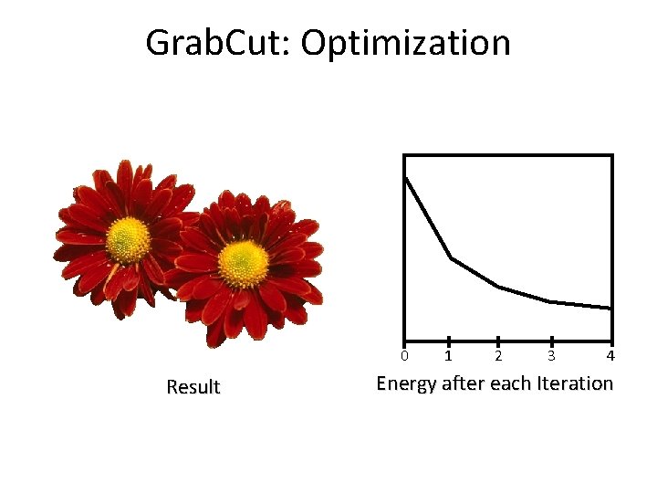
Grab. Cut: Optimization 0 Result 1 2 3 4 Energy after each Iteration

Grab. Cut: Optimization R Iterated graph cut Backgroun d Foreground & Background G R Backgroun d Foreground G

Summary – Intro: Probabilistic models – Two different approaches for learning – Generative/discriminative models, discriminative functions – Advanced segmentation system: Grab. Cut