Advanced Computer Vision Chapter 8 Dense Motion Estimation

Advanced Computer Vision Chapter 8 Dense Motion Estimation Presented by 王嘉会 and 傅楸善教授 E-mail: r 07945045@ntu. edu. tw Digital Camera and Computer Vision Laboratory Department of Computer Science and Information Engineering National Taiwan University, Taipei, Taiwan, R. O. C.

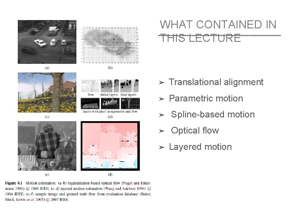
WHAT CONTAINED IN THIS LECTURE ➤ Translational alignment ➤ Parametric motion ➤ Spline-based motion ➤ Optical flow ➤ Layered motion

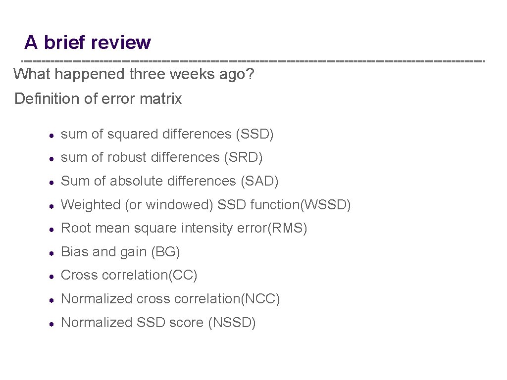
A brief review What happened three weeks ago? Definition of error matrix ● sum of squared differences (SSD) ● sum of robust differences (SRD) ● Sum of absolute differences (SAD) ● Weighted (or windowed) SSD function(WSSD) ● Root mean square intensity error(RMS) ● Bias and gain (BG) ● Cross correlation(CC) ● Normalized cross correlation(NCC) ● Normalized SSD score (NSSD)

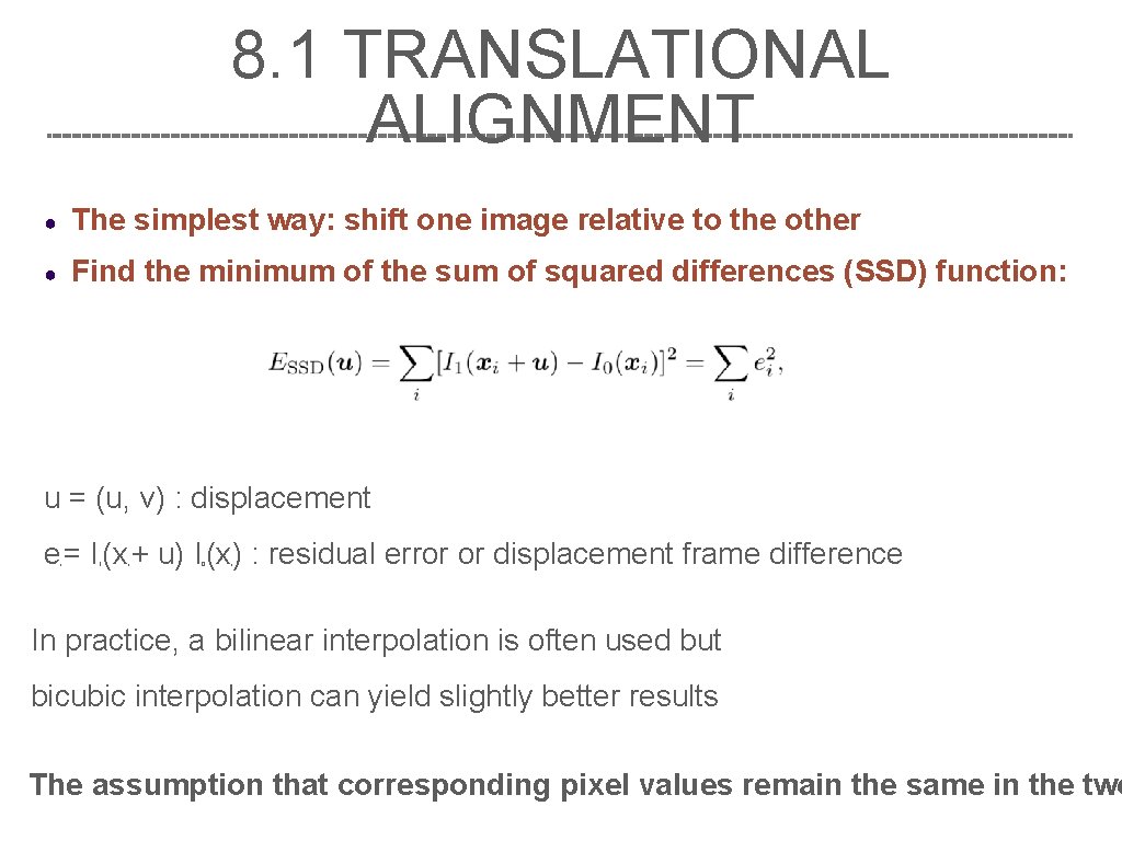
8. 1 TRANSLATIONAL ALIGNMENT ● The simplest way: shift one image relative to the other ● Find the minimum of the sum of squared differences (SSD) function: u = (u, v) : displacement e = I (x + u) I (x ) : residual error or displacement frame difference i 1 i 0 i In practice, a bilinear interpolation is often used but bicubic interpolation can yield slightly better results The assumption that corresponding pixel values remain the same in the two

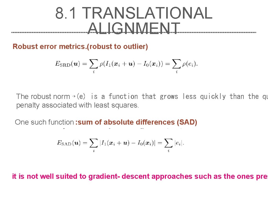
8. 1 TRANSLATIONAL ALIGNMENT Robust error metrics. (robust to outlier) The robust norm ⇢(e) is a function that grows less quickly than the qu penalty associated with least squares. One such function : sum of absolute differences (SAD) it is not well suited to gradient- descent approaches such as the ones pres

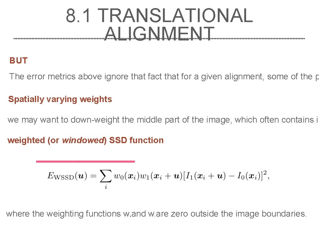
8. 1 TRANSLATIONAL ALIGNMENT BUT The error metrics above ignore that fact that for a given alignment, some of the p Spatially varying weights we may want to down-weight the middle part of the image, which often contains in weighted (or windowed) SSD function where the weighting functions w and w are zero outside the image boundaries. 0 1

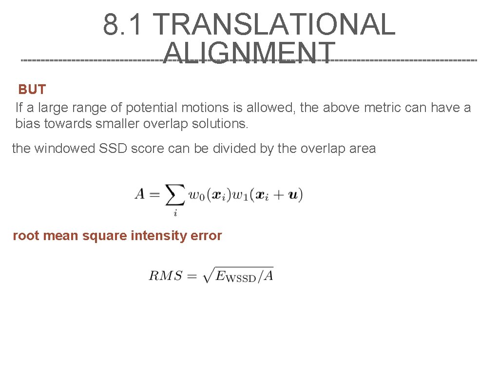
8. 1 TRANSLATIONAL ALIGNMENT BUT If a large range of potential motions is allowed, the above metric can have a bias towards smaller overlap solutions. the windowed SSD score can be divided by the overlap area root mean square intensity error

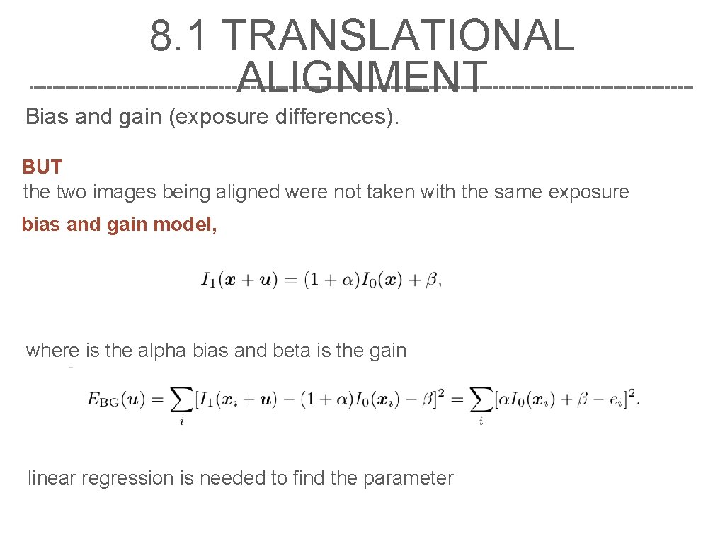
8. 1 TRANSLATIONAL ALIGNMENT Bias and gain (exposure differences). BUT the two images being aligned were not taken with the same exposure bias and gain model, where is the alpha bias and beta is the gain linear regression is needed to find the parameter

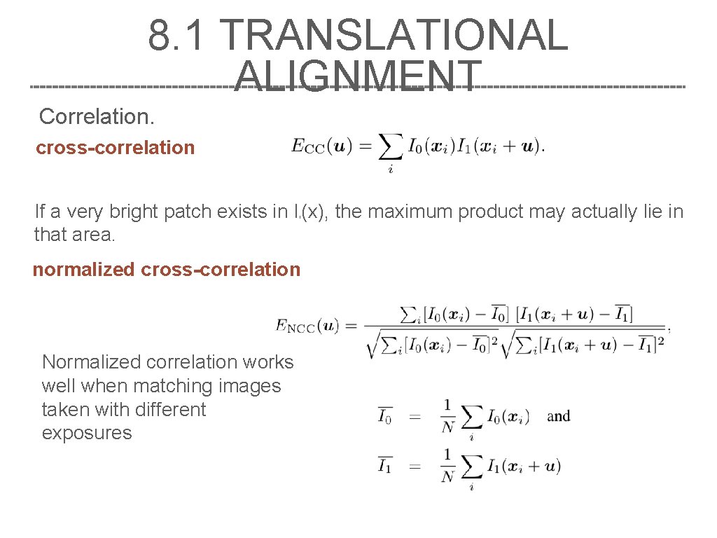
8. 1 TRANSLATIONAL ALIGNMENT Correlation. cross-correlation If a very bright patch exists in I (x), the maximum product may actually lie in that area. 1 normalized cross-correlation Normalized correlation works well when matching images taken with different exposures

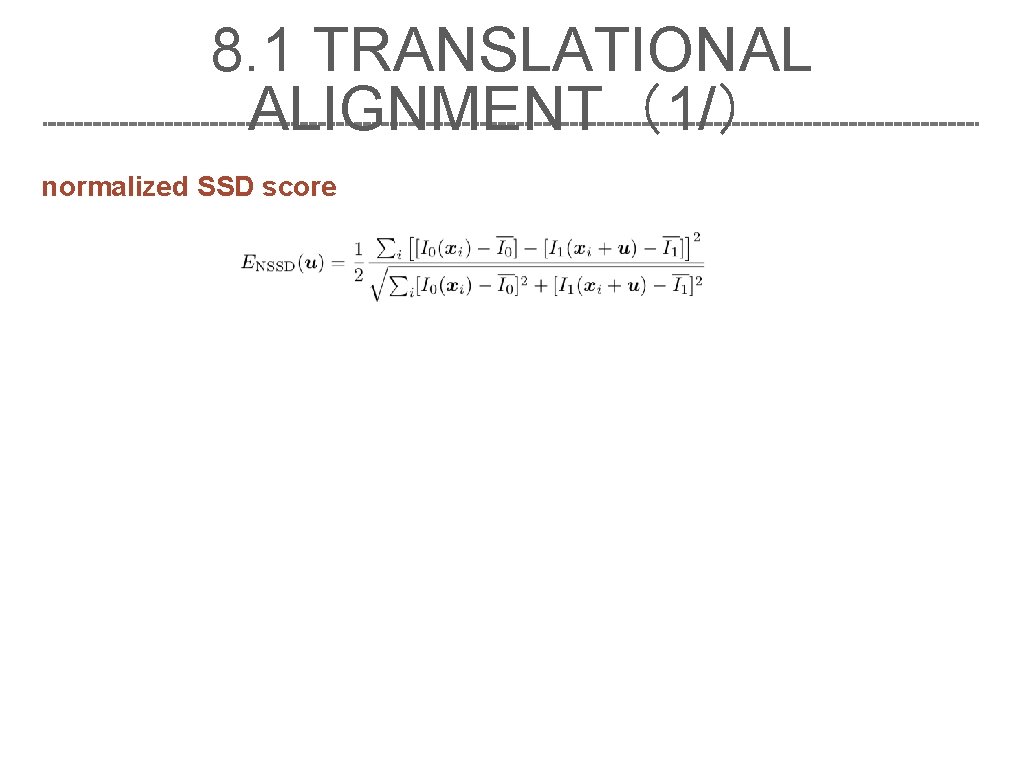
8. 1 TRANSLATIONAL ALIGNMENT（1/） normalized SSD score

JOKE

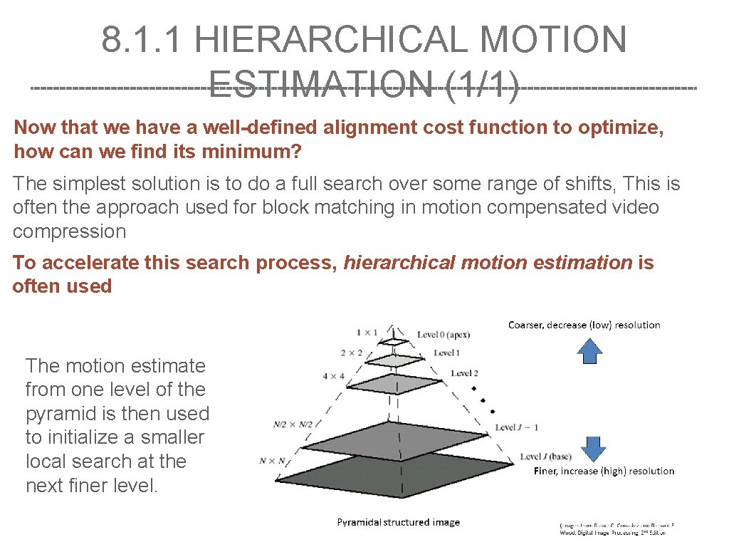
8. 1. 1 HIERARCHICAL MOTION ESTIMATION (1/1) Now that we have a well-defined alignment cost function to optimize, how can we find its minimum? The simplest solution is to do a full search over some range of shifts, This is often the approach used for block matching in motion compensated video compression To accelerate this search process, hierarchical motion estimation is often used The motion estimate from one level of the pyramid is then used to initialize a smaller local search at the next finer level.

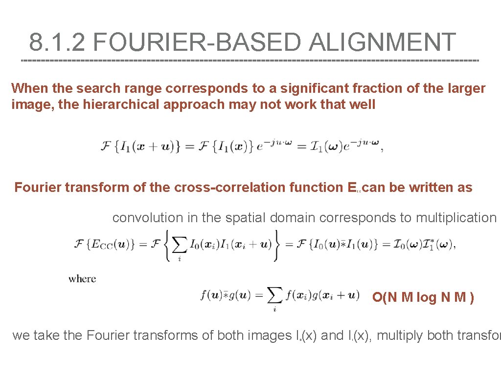
8. 1. 2 FOURIER-BASED ALIGNMENT When the search range corresponds to a significant fraction of the larger image, the hierarchical approach may not work that well Fourier transform of the cross-correlation function E can be written as CC convolution in the spatial domain corresponds to multiplication i O(N M log N M ) we take the Fourier transforms of both images I (x) and I (x), multiply both transfor 0 1

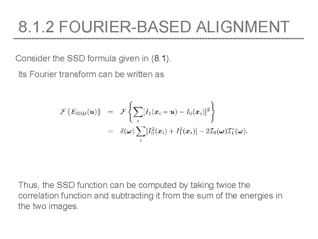
8. 1. 2 FOURIER-BASED ALIGNMENT Consider the SSD formula given in (8. 1). Its Fourier transform can be written as Thus, the SSD function can be computed by taking twice the correlation function and subtracting it from the sum of the energies in the two images.

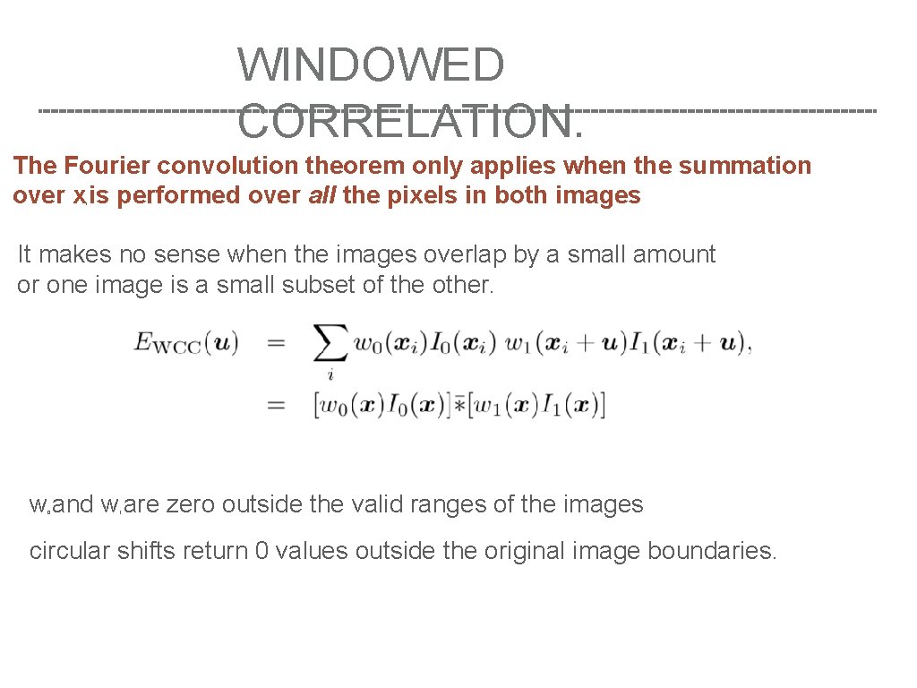
WINDOWED CORRELATION. The Fourier convolution theorem only applies when the summation over x is performed over all the pixels in both images i It makes no sense when the images overlap by a small amount or one image is a small subset of the other. w and w are zero outside the valid ranges of the images 0 1 circular shifts return 0 values outside the original image boundaries.

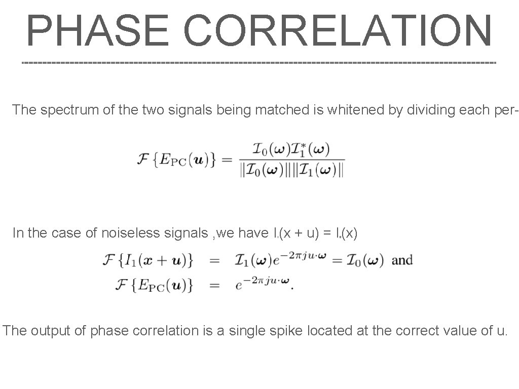
PHASE CORRELATION The spectrum of the two signals being matched is whitened by dividing each per- In the case of noiseless signals , we have I (x + u) = I (x) 1 0 The output of phase correlation is a single spike located at the correct value of u.

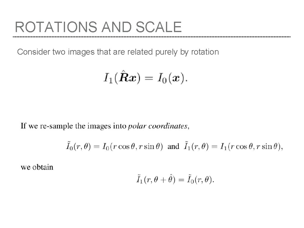
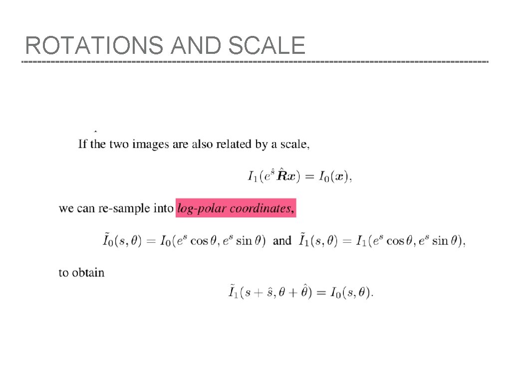
ROTATIONS AND SCALE Consider two images that are related purely by rotation

ROTATIONS AND SCALE

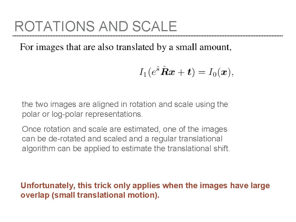
ROTATIONS AND SCALE the two images are aligned in rotation and scale using the polar or log-polar representations. Once rotation and scale are estimated, one of the images can be de-rotated and scaled and a regular translational algorithm can be applied to estimate the translational shift. Unfortunately, this trick only applies when the images have large overlap (small translational motion).

JOKE

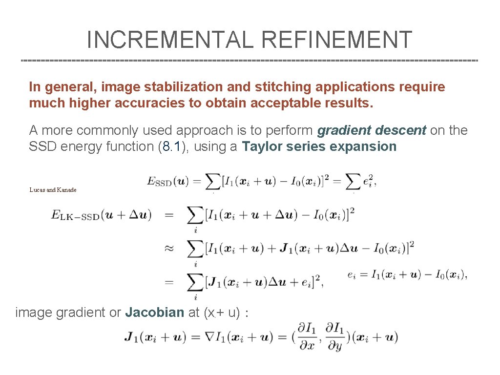
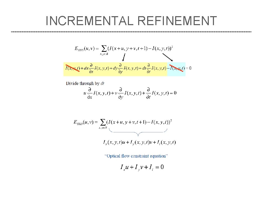
INCREMENTAL REFINEMENT In general, image stabilization and stitching applications require much higher accuracies to obtain acceptable results. A more commonly used approach is to perform gradient descent on the SSD energy function (8. 1), using a Taylor series expansion Lucas and Kanade image gradient or Jacobian at (x + u)： i

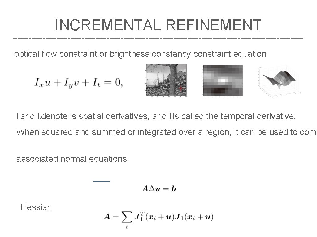
INCREMENTAL REFINEMENT optical flow constraint or brightness constancy constraint equation I and I denote is spatial derivatives, and I is called the temporal derivative. x y t When squared and summed or integrated over a region, it can be used to comp associated normal equations Hessian

INCREMENTAL REFINEMENT

INCREMENTAL REFINEMENT optical flow constraint or brightness constancy constraint equation I and I denote is spatial derivatives, and I is called the temporal derivative. x y t When squared and summed or integrated over a region, it can be used to comp associated normal equations Hessian

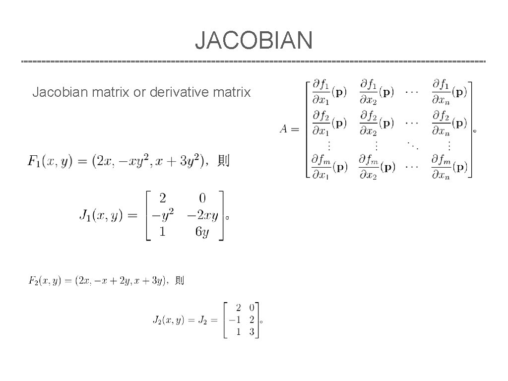
JACOBIAN Jacobian matrix or derivative matrix

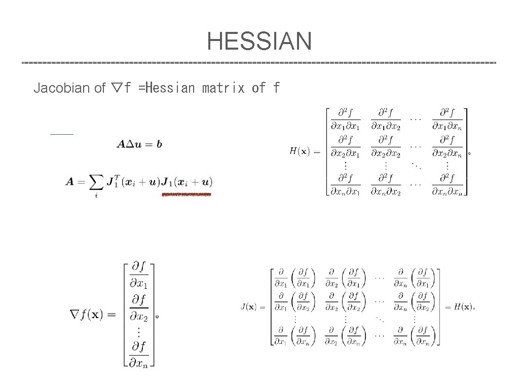
HESSIAN Jacobian of ▽f =Hessian matrix of f

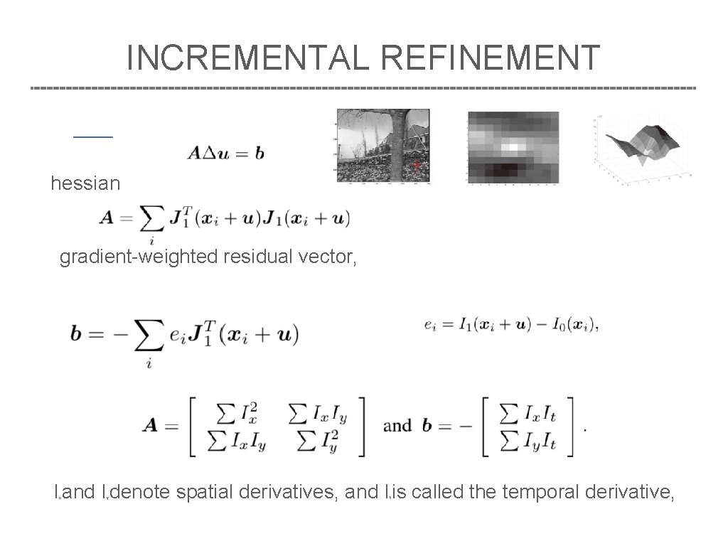
INCREMENTAL REFINEMENT hessian gradient-weighted residual vector, I and I denote spatial derivatives, and I is called the temporal derivative, x y t

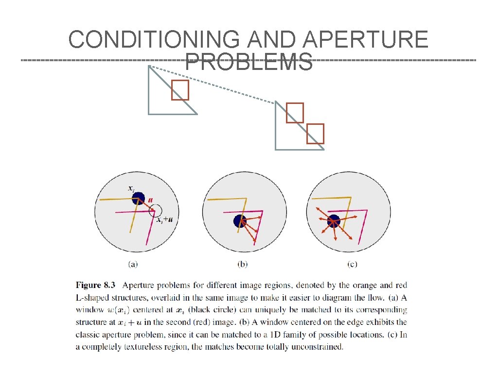
CONDITIONING AND APERTURE PROBLEMS

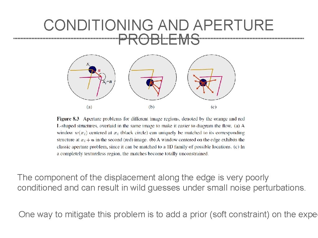
CONDITIONING AND APERTURE PROBLEMS The component of the displacement along the edge is very poorly conditioned and can result in wild guesses under small noise perturbations. One way to mitigate this problem is to add a prior (soft constraint) on the expec

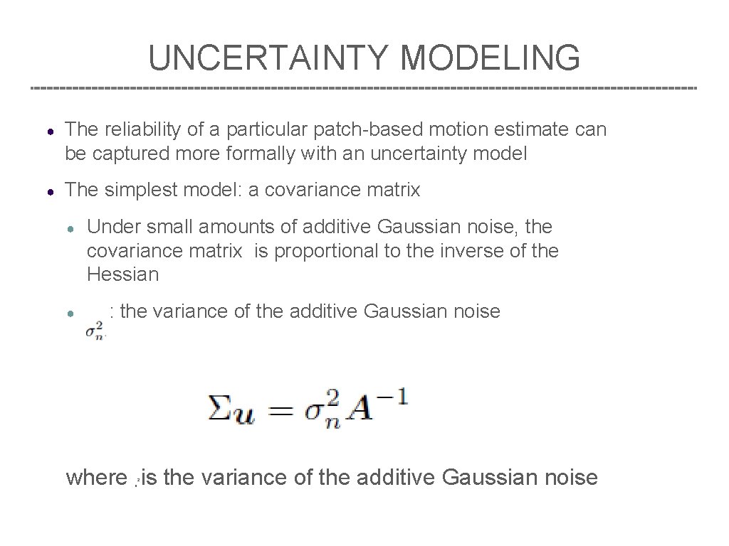
UNCERTAINTY MODELING ● The reliability of a particular patch-based motion estimate can be captured more formally with an uncertainty model ● The simplest model: a covariance matrix ● ● Under small amounts of additive Gaussian noise, the covariance matrix is proportional to the inverse of the Hessian : the variance of the additive Gaussian noise where is the variance of the additive Gaussian noise 2 n

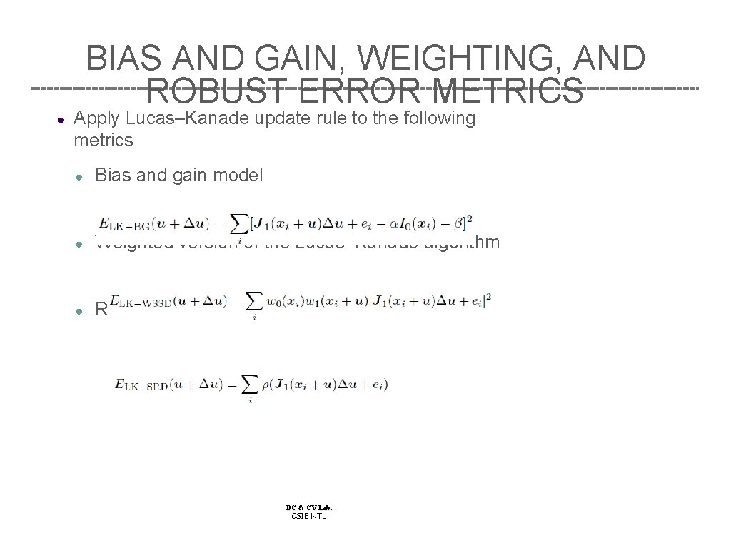
BIAS AND GAIN, WEIGHTING, AND ROBUST ERROR METRICS ● Apply Lucas–Kanade update rule to the following metrics ● Bias and gain model ● Weighted version of the Lucas–Kanade algorithm ● Robust error metric DC & CV Lab. CSIE NTU

JOKE

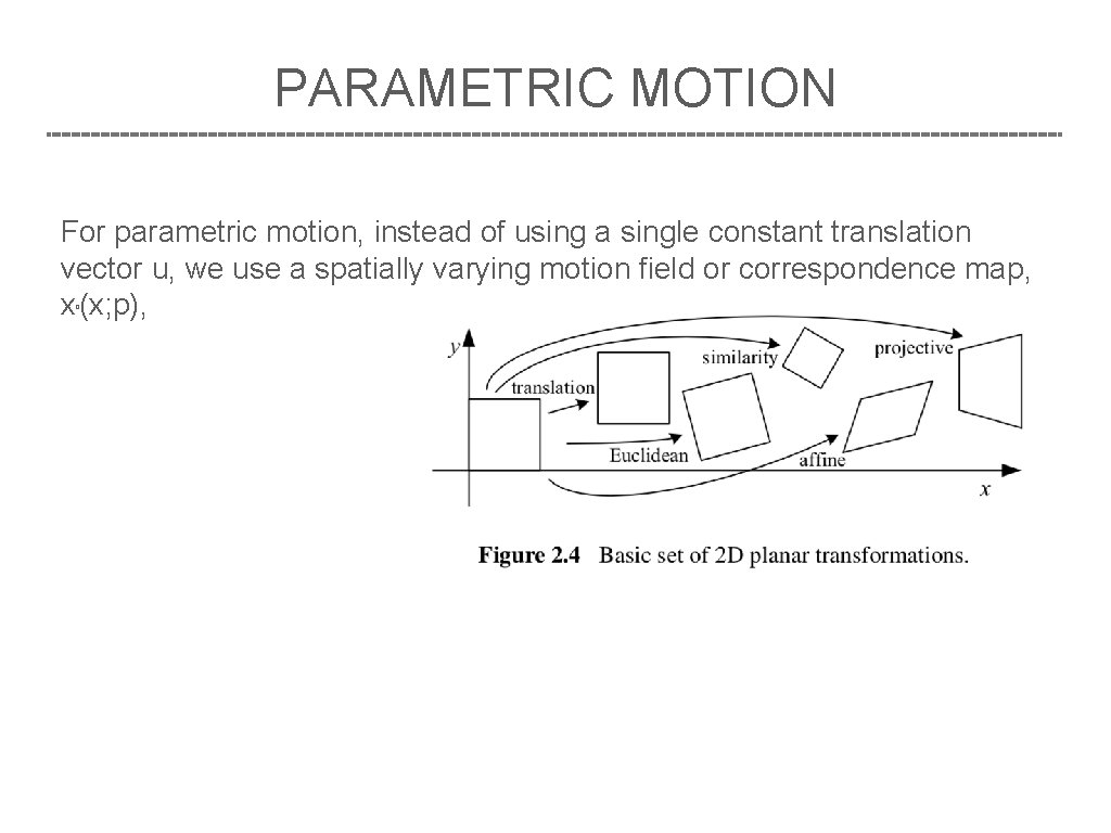
PARAMETRIC MOTION For parametric motion, instead of using a single constant translation vector u, we use a spatially varying motion field or correspondence map, x (x; p), 0

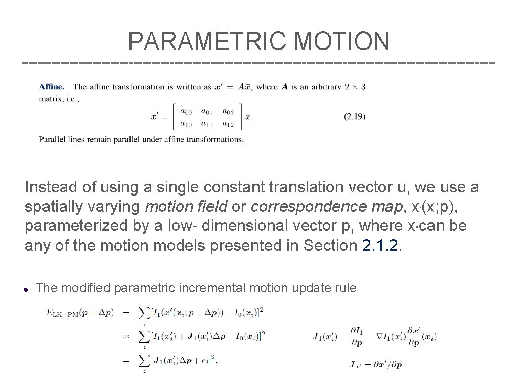
PARAMETRIC MOTION Instead of using a single constant translation vector u, we use a spatially varying motion field or correspondence map, x (x; p), parameterized by a low- dimensional vector p, where x can be any of the motion models presented in Section 2. 1. 2. 0 0 ● The modified parametric incremental motion update rule

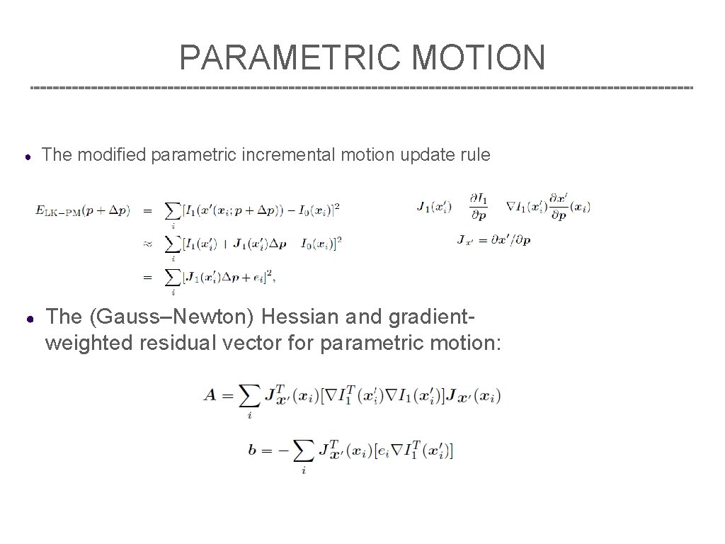
PARAMETRIC MOTION ● ● The modified parametric incremental motion update rule The (Gauss–Newton) Hessian and gradientweighted residual vector for parametric motion:

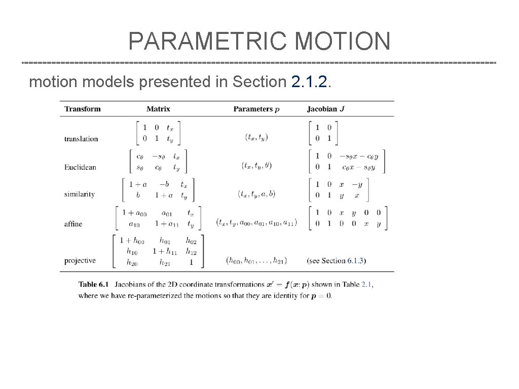
PARAMETRIC MOTION motion models presented in Section 2. 1. 2.

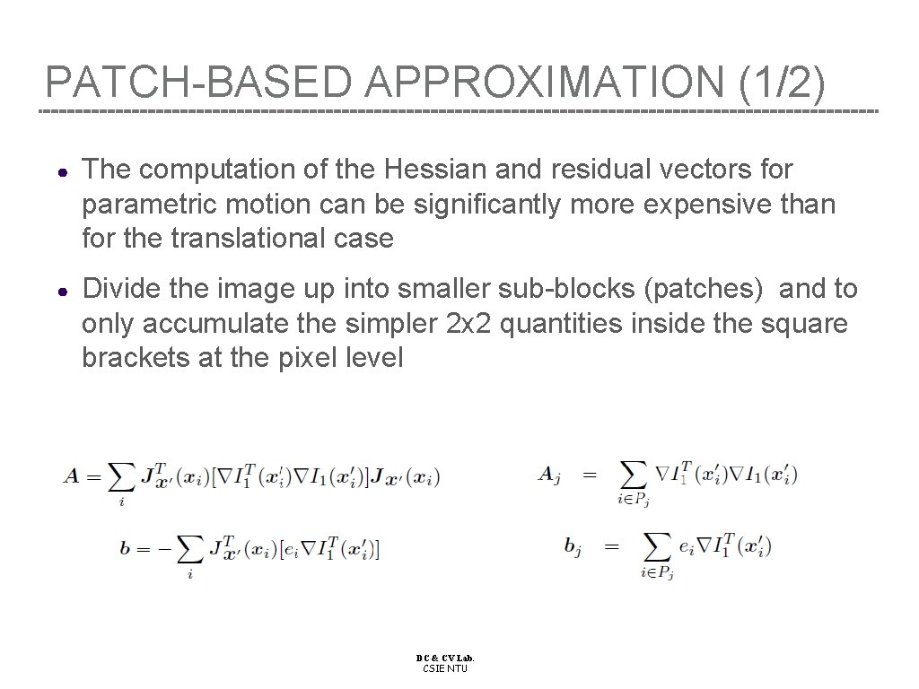
PATCH-BASED APPROXIMATION (1/2) ● The computation of the Hessian and residual vectors for parametric motion can be significantly more expensive than for the translational case ● Divide the image up into smaller sub-blocks (patches) and to only accumulate the simpler 2 x 2 quantities inside the square brackets at the pixel level DC & CV Lab. CSIE NTU

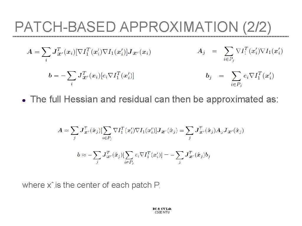
PATCH-BASED APPROXIMATION (2/2) ● The full Hessian and residual can then be approximated as: where xˆ is the center of each patch P j j DC & CV Lab. CSIE NTU

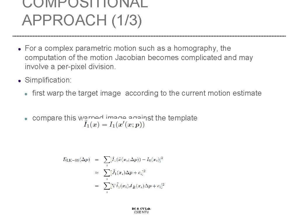
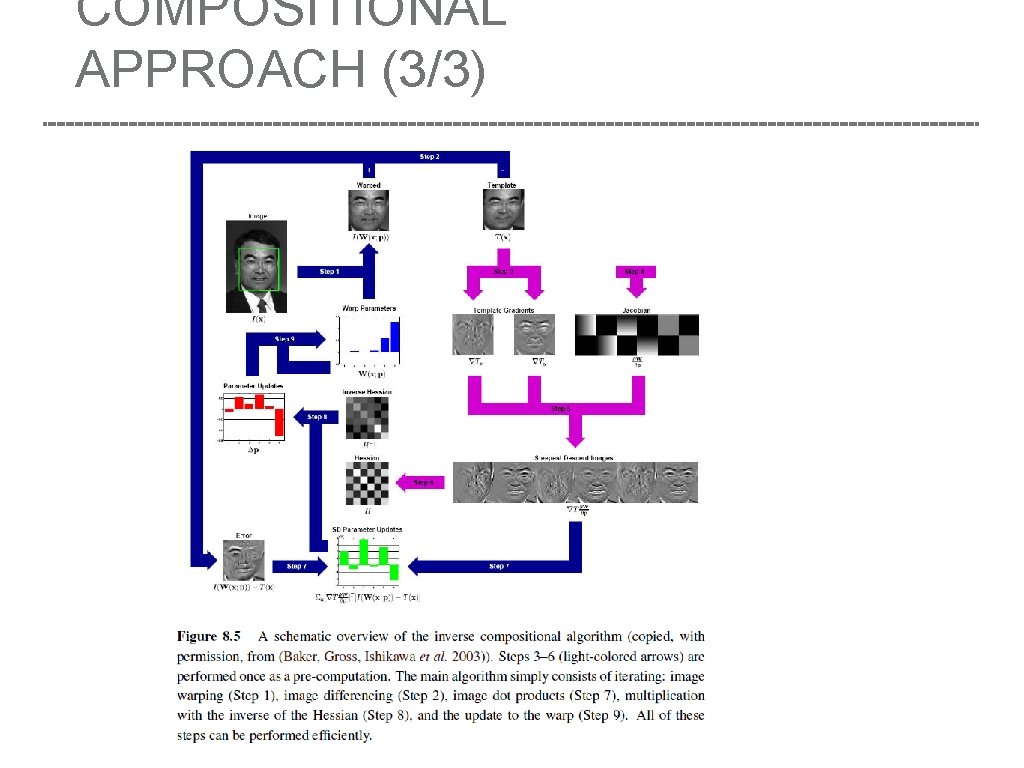
COMPOSITIONAL APPROACH (1/3) ● For a complex parametric motion such as a homography, the computation of the motion Jacobian becomes complicated and may involve a per-pixel division. ● Simplification: ● first warp the target image according to the current motion estimate ● compare this warped image against the template DC & CV Lab. CSIE NTU

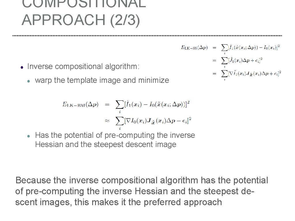
COMPOSITIONAL APPROACH (2/3) ● Inverse compositional algorithm: ● warp the template image and minimize ● Has the potential of pre-computing the inverse Hessian and the steepest descent image Because the inverse compositional algorithm has the potential of pre-computing the inverse Hessian and the steepest descent images, this makes it the preferred approach

COMPOSITIONAL APPROACH (3/3)

8. 2. 1 APPLICATION: VIDEO STABILIZATION Algorithms for stabilization run inside both hardware devices, Three major stages of stabilization, namely motion estimation, motion smooth Motion estimation algorithms lock onto the background motion, which is a result of the camera movement, without getting distracted by independent moving foreground objects. Motion smoothing algorithms recover the low-frequency (slowly varying) part of the motion and then estimate the high-frequency shake component that needs to be removed. Finally, image warping algorithms apply the high-frequency correction to render the original frames as if the camera had undergone only the smooth motion.

JOKE

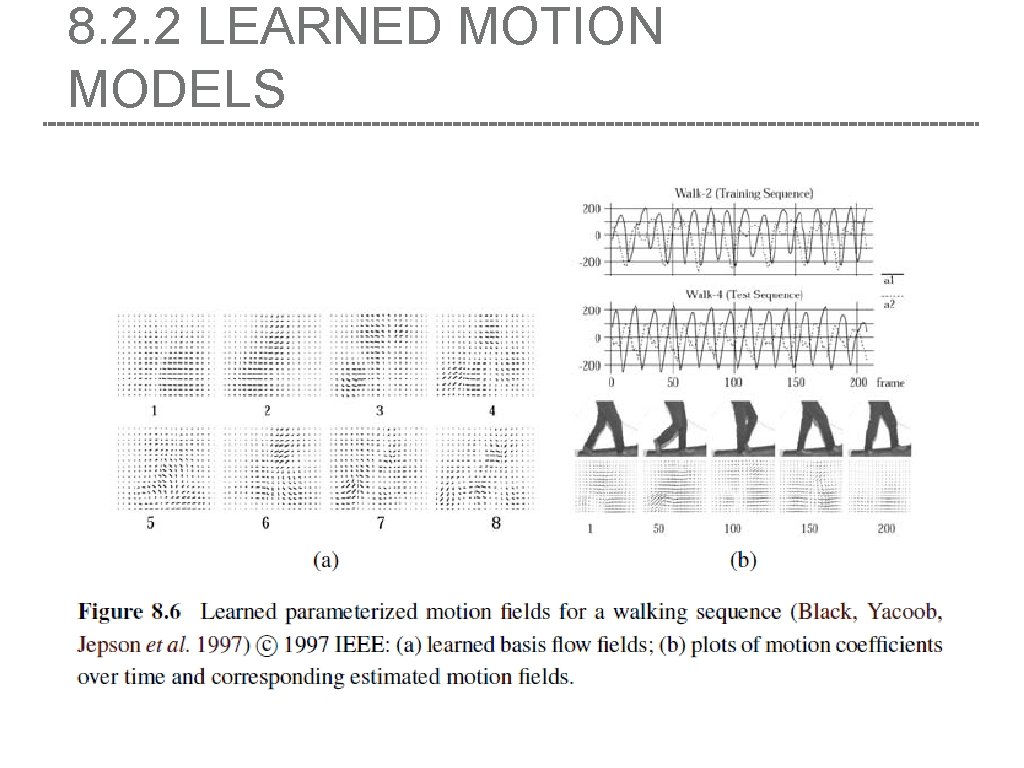
8. 2. 2 LEARNED MOTION MODELS • First, a set of dense motion fields (Section 8. 4) is computed from a set of training videos. • Next, singular value decomposition (SVD) is applied to the stack of motion fields u (x) to compute the first few singular vectors v (x). t k • Finally, for a new test sequence, a novel flow field is computed using a coarse-to-fine algorithm that estimates the unknown coefficient a in the parameterized flow field k

8. 2. 2 LEARNED MOTION MODELS

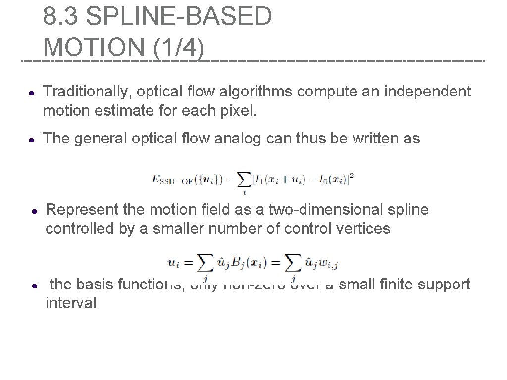
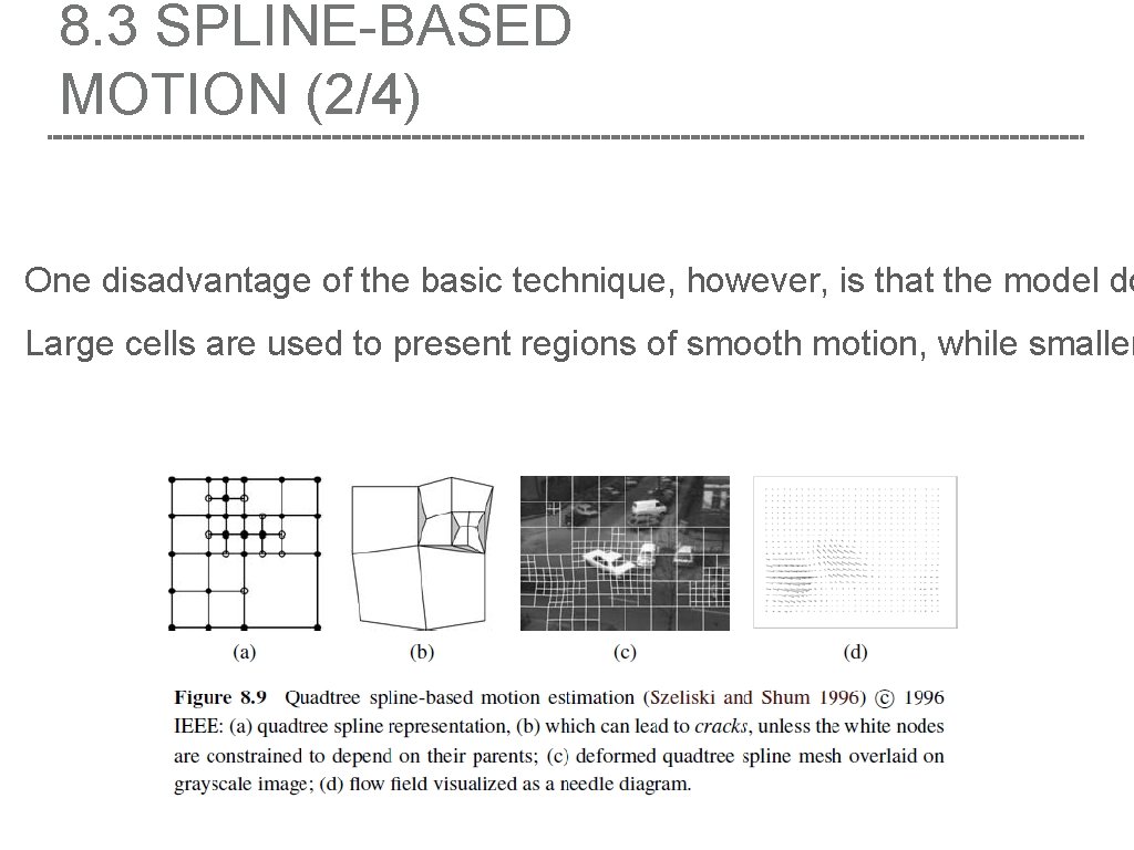
8. 3 SPLINE-BASED MOTION (1/4) ● Traditionally, optical flow algorithms compute an independent motion estimate for each pixel. ● The general optical flow analog can thus be written as ● Represent the motion field as a two-dimensional spline controlled by a smaller number of control vertices ● the basis functions; only non-zero over a small finite support interval

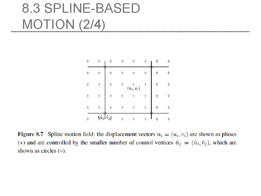
8. 3 SPLINE-BASED MOTION (2/4)

8. 3 SPLINE-BASED MOTION (1/4) ● Traditionally, optical flow algorithms compute an independent motion estimate for each pixel. ● The general optical flow analog can thus be written as ● Represent the motion field as a two-dimensional spline controlled by a smaller number of control vertices ● the basis functions; only non-zero over a small finite support interval

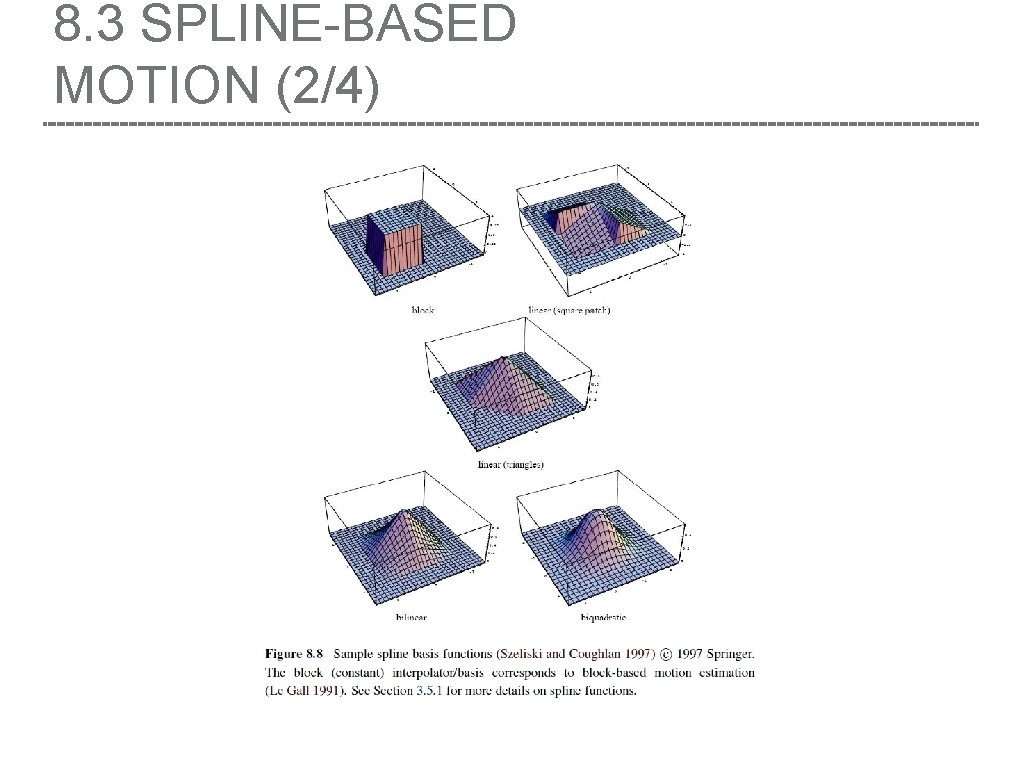
8. 3 SPLINE-BASED MOTION (1/4) • where the B (x ) are called the basis functions and are only non-zero over a small finite sup- port interval. j i • We call the w = B (x ) weights to emphasize that the {u } are known linear combinations of the {uˆ }. ij j i i j • Some commonly used spline basis functions are shown below

8. 3 SPLINE-BASED MOTION (2/4)

8. 3 SPLINE-BASED MOTION (2/4) One disadvantage of the basic technique, however, is that the model do Large cells are used to present regions of smooth motion, while smaller

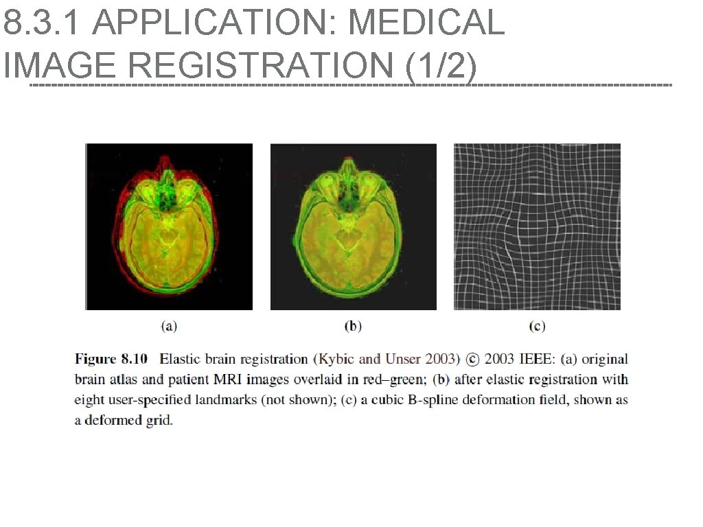
8. 3. 1 APPLICATION: MEDICAL IMAGE REGISTRATION (1/2)

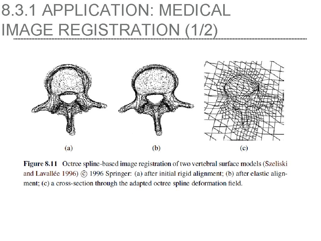
8. 3. 1 APPLICATION: MEDICAL IMAGE REGISTRATION (1/2)

JOKE

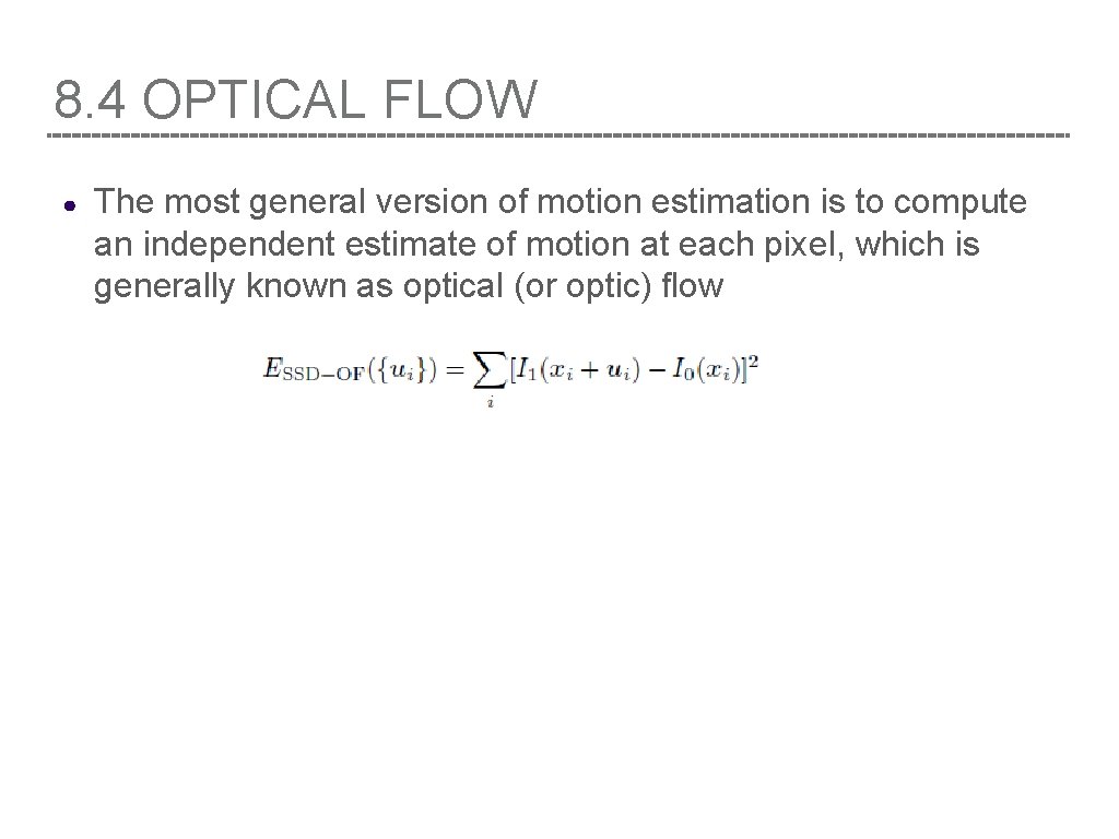
8. 4 OPTICAL FLOW ● The most general version of motion estimation is to compute an independent estimate of motion at each pixel, which is generally known as optical (or optic) flow

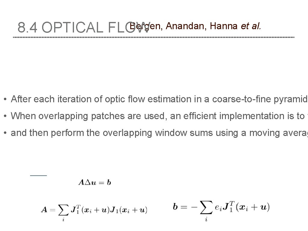
Bergen, Anandan, Hanna et al. 8. 4 OPTICAL FLOW • After each iteration of optic flow estimation in a coarse-to-fine pyramid • When overlapping patches are used, an efficient implementation is to f • and then perform the overlapping window sums using a moving averag

8. 4 OPTICAL Horn and Schunck FLOW HW assign

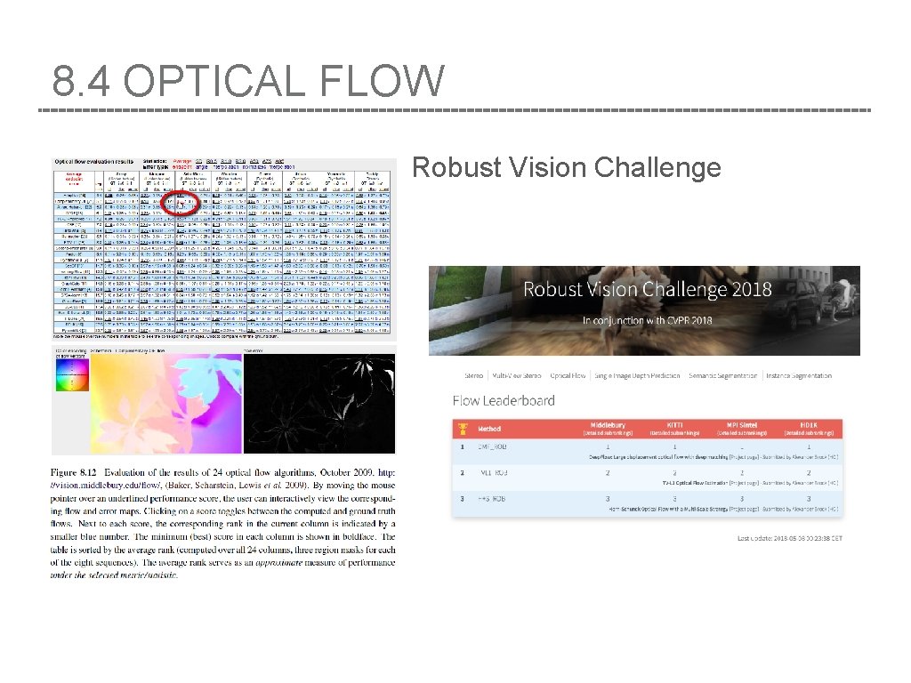
8. 4 OPTICAL FLOW Robust Vision Challenge

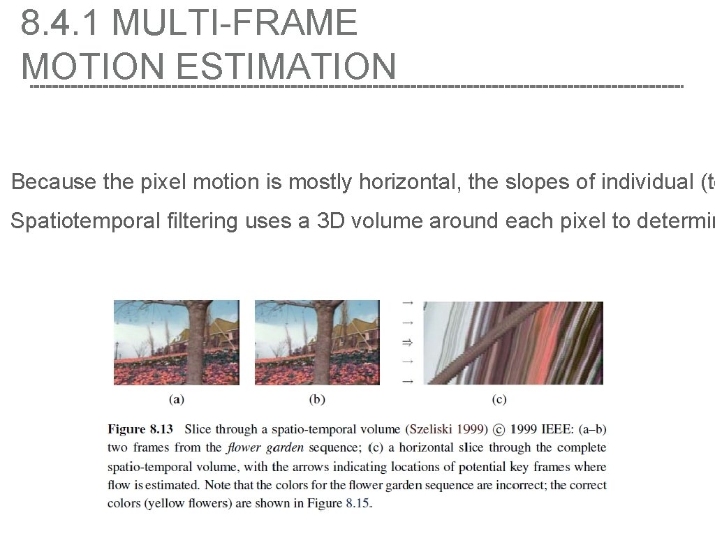
8. 4. 1 MULTI-FRAME MOTION ESTIMATION So far, we have looked at motion estimation as a two-frame problem, where the goal is to compute a motion field that aligns pixels from one image with those in another. In practice, motion estimation is usually applied to video, where a whole sequence of frames is available to perform this task. One classic approach to multi-frame motion is to filter the spatiotempor

8. 4. 1 MULTI-FRAME MOTION ESTIMATION Because the pixel motion is mostly horizontal, the slopes of individual (te Spatiotemporal filtering uses a 3 D volume around each pixel to determin

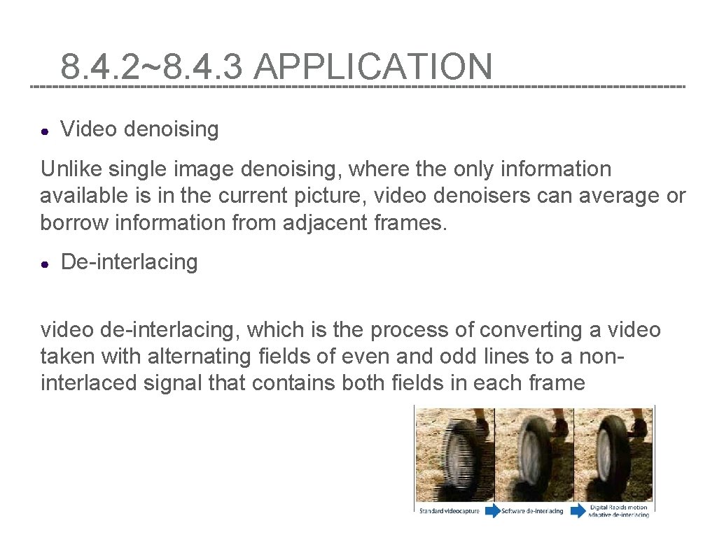
8. 4. 2~8. 4. 3 APPLICATION ● Video denoising Unlike single image denoising, where the only information available is in the current picture, video denoisers can average or borrow information from adjacent frames. ● De-interlacing video de-interlacing, which is the process of converting a video taken with alternating fields of even and odd lines to a noninterlaced signal that contains both fields in each frame

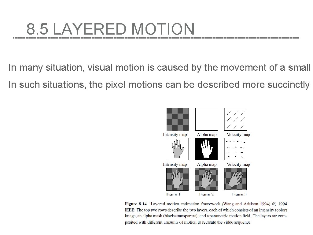
8. 5 LAYERED MOTION In many situation, visual motion is caused by the movement of a small In such situations, the pixel motions can be described more succinctly (

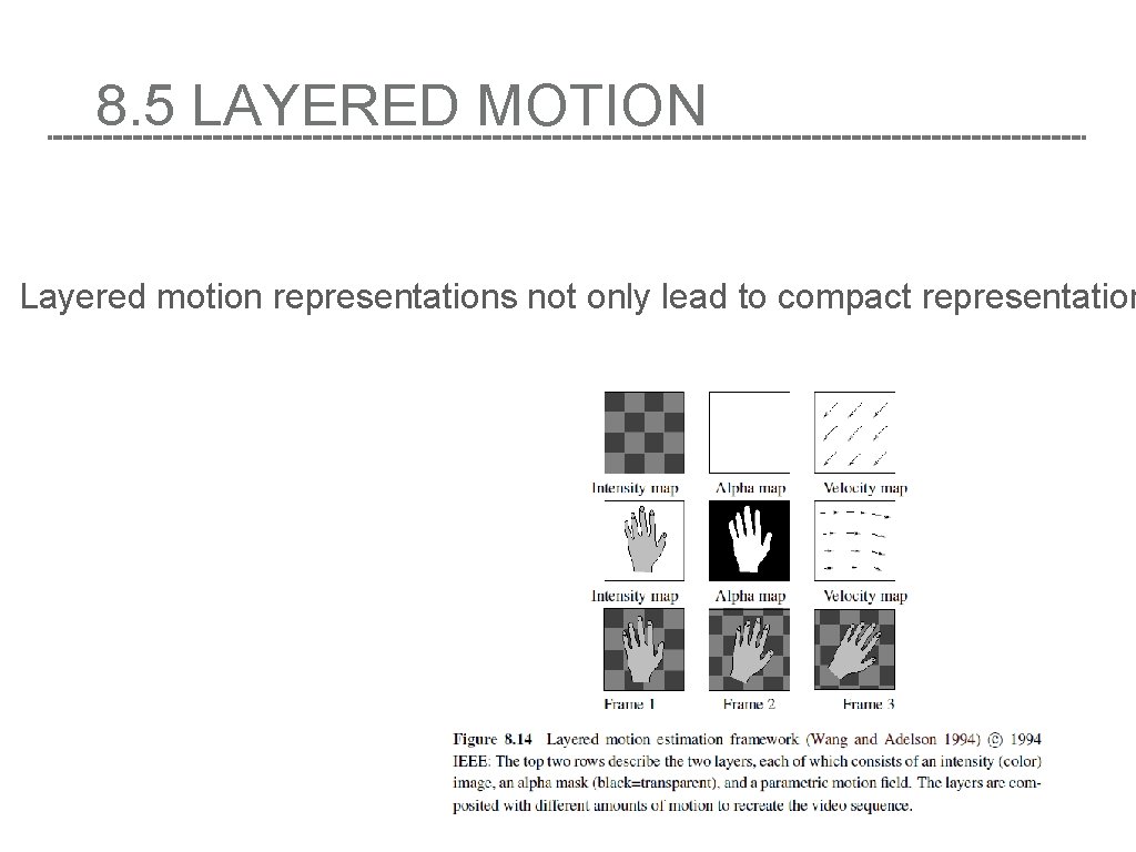
8. 5 LAYERED MOTION Layered motion representations not only lead to compact representation

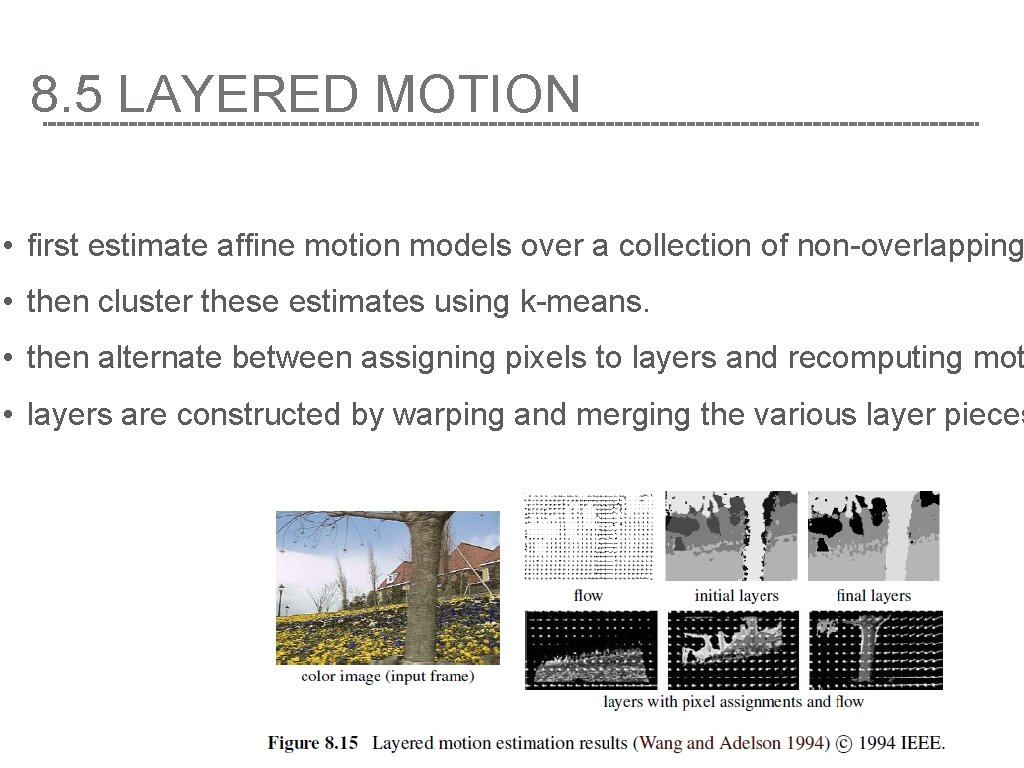
8. 5 LAYERED MOTION • first estimate affine motion models over a collection of non-overlapping • then cluster these estimates using k-means. • then alternate between assigning pixels to layers and recomputing mot • layers are constructed by warping and merging the various layer pieces

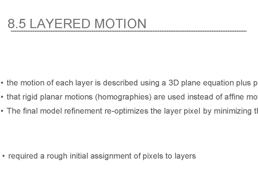
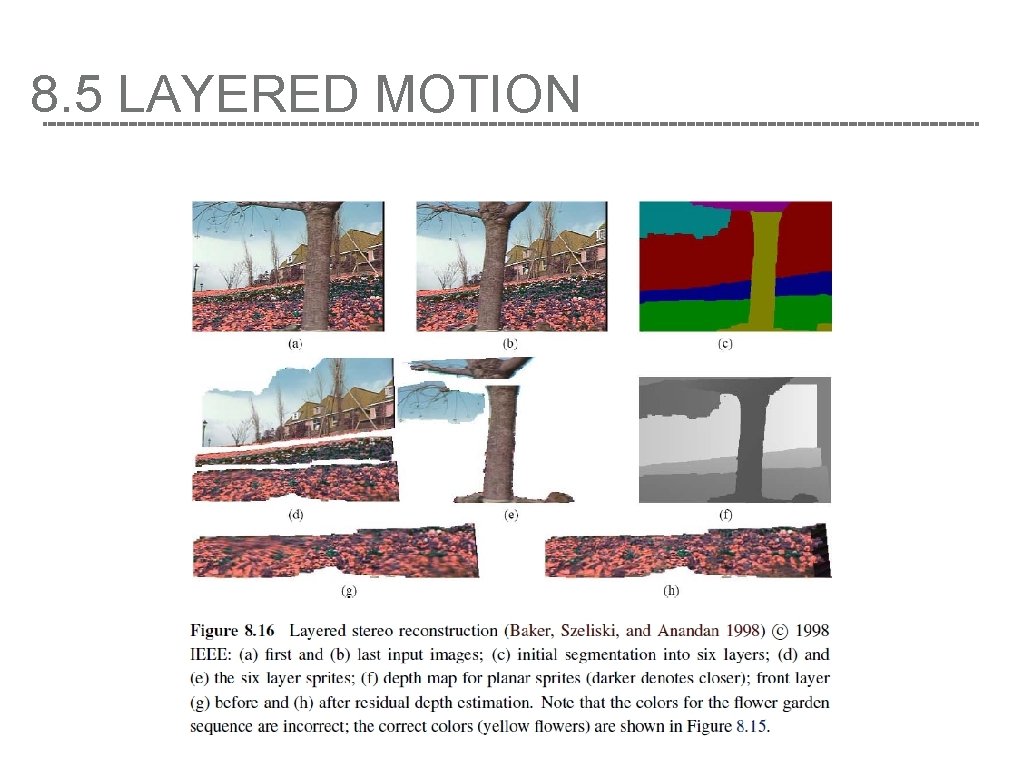
8. 5 LAYERED MOTION • the motion of each layer is described using a 3 D plane equation plus pe • that rigid planar motions (homographies) are used instead of affine mot • The final model refinement re-optimizes the layer pixel by minimizing th • required a rough initial assignment of pixels to layers

8. 5 LAYERED MOTION

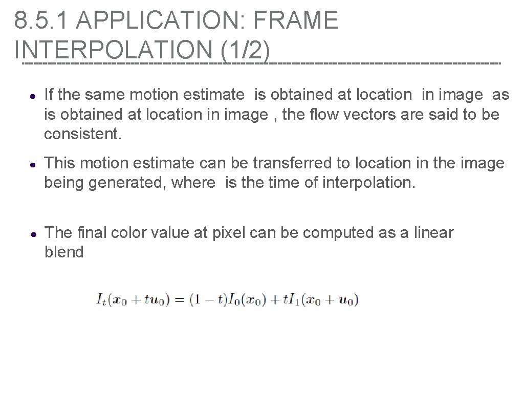
8. 5. 1 APPLICATION: FRAME INTERPOLATION (1/2) ● If the same motion estimate is obtained at location in image as is obtained at location in image , the flow vectors are said to be consistent. ● This motion estimate can be transferred to location in the image being generated, where is the time of interpolation. ● The final color value at pixel can be computed as a linear blend

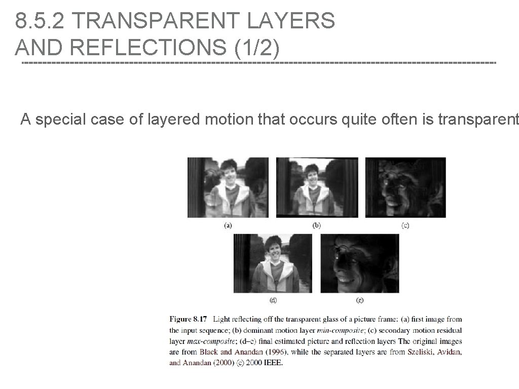
8. 5. 2 TRANSPARENT LAYERS AND REFLECTIONS (1/2) A special case of layered motion that occurs quite often is transparent

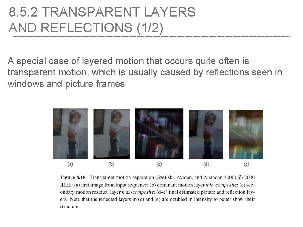
8. 5. 2 TRANSPARENT LAYERS AND REFLECTIONS (1/2) A special case of layered motion that occurs quite often is transparent motion, which is usually caused by reflections seen in windows and picture frames

JOKE