Advanced Computer Vision Chapter 7 Feature Detection and

Advanced Computer Vision Chapter 7 Feature Detection and Matching Presented by: 傅楸善 & 孫譽 yu. sun 1997@gmail. com 0928572743

Feature Detection and Matching (1/4) • • • 7. 1 Points and patches 7. 2 Edges and contours 7. 3 Contour tracking 7. 4 Lines and vanishing points 7. 5 Segmentation

Feature Detection and Matching (2/4)

Feature Detection and Matching (3/4)

Feature Detection and Matching (4/4)

7. 1 Points and Patches (1/4) • There are two main approaches: – Find features in one image that can be accurately tracked using a local search technique. (e. g. , video sequences) – Independently detect features in all the images under consideration and then match features based on their local appearance. (e. g. , stitching panoramas, establishing correspondences)

7. 1 Points and Patches (2/4) • Video sequences

7. 1 Points and Patches (3/4) • Stitching panorama

Points and Patches (4/4) • Three stages: – Feature detection (extraction) stage – Feature description stage – Feature matching stage or Feature Tracking stage

7. 1. 1 Feature Detectors

Aperture Problem

Aperture Problem

Weighted Summed Square Difference • • I 0, I 1: the two images being compared u: the displacement vector w(x): spatially varying weighting function summation i: over all the pixels in the patch

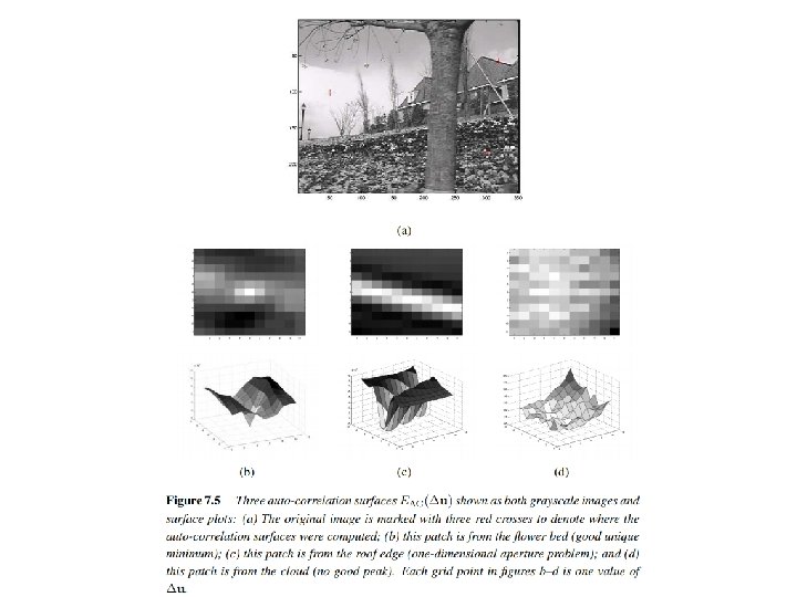
Auto-correlation Function or Surface • • I 0: the image being compared ∆u: small variations in position w(x): spatially varying weighting function summation i: over all the pixels in the patch

Approximation of Auto-correlation Function (1/3) • I 0(xi+ ∆u) ≈ I 0(xi) + ∇ I 0(xi)．∆u • ∇ I 0(xi): image gradient at xi

Approximation of Auto-correlation Function (2/3) • Auto-correlation matrix A: • w: weighting kernel (from spatially varying weighting function) • Ix, Iy: horizontal and vertical derivatives of Gaussians Schmid, C. , Mohr, R. , and Bauckhage, C. (2000). Evaluation of interest point detectors. International Journal of Computer Vision, 37(2): 151– 172.

Approximation of Auto-correlation Function (3/3) • Assume (λ 0, λ 1) are two eigenvalues of A and λ 0 <= λ 1. • Since the larger uncertainty depends on the smaller eigenvalue, it makes sense to find maxima in the smaller eigenvalue to locate good features to track.

Approximation of Auto-correlation Function

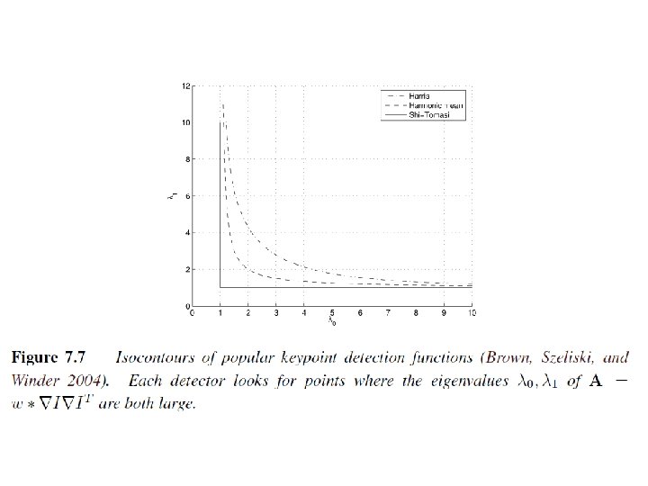
Other Measurements (1/3) • Quantity proposed by Harris and Stephens: • α = 0. 06 • No square roots • It is still rotationally invariant and downweights edge-like features when λ 1 >> λ 0.

Other Measurements (2/3) • Triggs(2004) • α = 0. 05

Other Measurements (3/3) • Quantity proposed by Brown, Szeliski, and Winder: • It can be used when λ 1 ≈ λ 0.

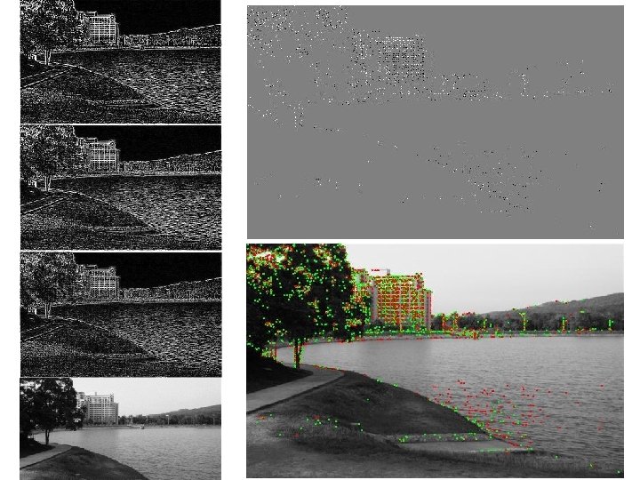
Basic Feature Detection Algorithm (1/2) • Step 1: Compute the horizontal and vertical derivatives of the image Ix and Iy by convolving the original image with derivatives of Gaussians. • Step 2: Compute three images (Ix 2, Iy 2, Ix. Iy) corresponding to the outer products of these gradients.

Basic Feature Detection Algorithm (2/2) • Step 3: Convolve each of these images with a larger Gaussian (the weighting kernel). • Step 4: Compute a scalar interest measure using one of the formulas discussed above. • Step 5: Find local maxima above a certain threshold and report them as detected feature point locations.

Adaptive Non-maximal Suppression (ANMS) (1/2) • Simply finding local maxima -> uneven distribution of feature points • Detect features that are: – Local maxima – Response value is greater than all of its neighbors within a radius r

Adaptive Non-maximal Suppression (ANMS) (2/2)

Measuring Repeatability • Which feature points should we use among the large number of detected feature points? • Measure repeatability after applying rotations, scale changes, illumination changes, viewpoint changes, and adding noise.

Scale Invariance (1/2) • Problem: if no good feature points in image? • Solution: multi-scale

Scale Invariance (2/2) Do. G: Difference of Gaussian

Rotational Invariance

Affine Invariance

Maximally Stable Extremal Region (MSER) • Only work for grayscale images • Incrementally add pixels as the threshold is changed. • Maximally stable: changing rate of area with respect to the threshold is minimal

Recent Papers • Learning covariant feature detectors (Lenc and Vedaldi 2016); • Learning to assign orientations to feature points (Yi, Verdie et al. 2016); • LIFT, learned invariant feature transforms (Yi, Trulls et al. 2016), • Super. Point, self-supervised interest point detection and description (De. Tone, Malisiewicz, and Rabinovich 2018), and • LF-Net, learning local features from images (Ono, Trulls et al. 2018), all three of which • jointly optimize the detectors and descriptors in a single (multi-head) pipeline;

7. 1. 2 Feature Descriptors • Sum of squared difference • Normalized cross-correlation (Chapter 9)

Scale Invariant Feature Transform (SIFT)

Multi-scale Oriented Patches (MOP) • • • Simpler SIFT, without every scale Do. Gs Used on image stitching, and so on Detector: Harris corner detector Multi-scale -> make program robust Do. G: Difference of Gaussian

Multi-scale Oriented Patches (MOP)

Orientation Estimation

Orientation Estimation

Gradient Location-orientation Histogram (GLOH)

7. 1. 3 Feature Matching • Two subjects: – select a matching strategy – devise efficient data structures and algorithms to perform this matching

Matching Strategy (1/4) • Simplest method: set a distance threshold and match within this threshold.

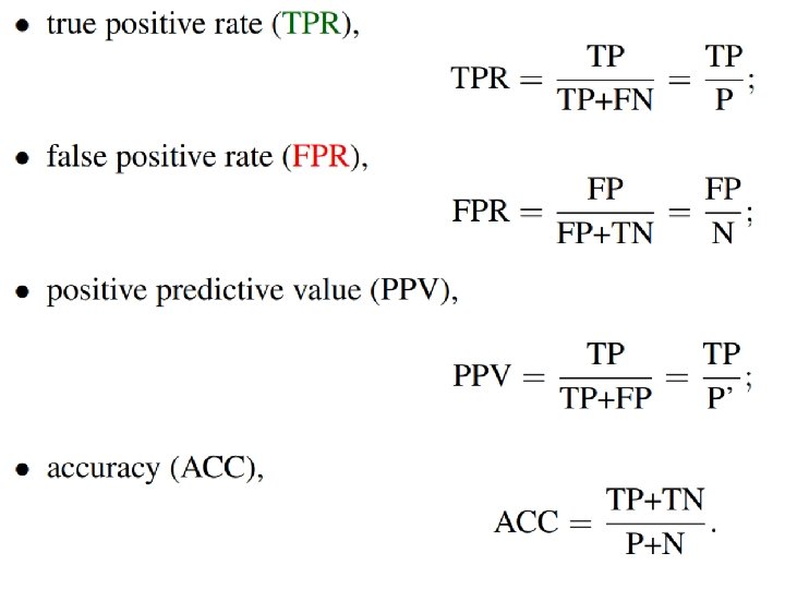
Matching Strategy (2/4) • Confusion matrix to estimate performance:

Matching Strategy (3/4) ROC: Receiver Operating Characteristic

Matching Strategy (4/4) • Indexing structures: – Multi-dimensional search tree – Multi-dimensional hashing

7. 1. 4 Feature Tracking (1/3) • To find a set of likely feature locations in a first image and to then search for their corresponding locations in subsequent images. • Expected amount of motion and appearance deformation between adjacent frames is expected to be small.

Feature Tracking (2/3) • Selecting good features to track is closely related to selecting good features to match. • When searching corresponding patch, weighted summed square difference works well enough.

Feature Tracking (3/3) • If features are being tracked over longer image sequences, their appearance can undergo larger changes. – Continuously match against the originally detected feature – Re-sample each subsequent frame at the matching location – Use affine motion model to measure dissimilarity (ex: Kanade–Lucas–Tomasi (KLT) tracker)

7. 2 Edges (1/2) • What are edges in image: – The boundaries of objects – Occlusion events in 3 D – Shadow boundaries or crease edges – Grouped into longer curves or contours

Edges (2/2)

7. 2. 1 Edge Detection (1/3) • Edge has rapid intensity variation. – J: local gradient vector Its direction is perpendicular to the edge, and its magnitude is the intensity variation. – I: original image

Edge Detection (2/3) • Taking image derivatives makes noise larger. • Use Gaussian filter to remove noise: – G: Gaussian filter – σ: width of Gaussian filter

Edge Detection (3/3) • To thin such a continuous gradient image to only return isolated edges: • Use Laplacian of Gaussian: – S: second gradient operator • Then find the zero crossings to get the maximum of gradient.

Scale Selection

Color Edge Detection • Band separation and combination -> not good

7. 3 Lines • Man-made world is full of straight lines, so detecting and matching these lines can be useful in a variety of applications.

7. 3. 1 Successive Approximation • Line simplification: – Piecewise-linear polyline – B-spline curve

7. 3. 2 Hough Transforms (1/2) • Original Hough transforms:

Hough Transforms (2/2) • Oriented Hough transform:

Hough Transforms Algorithm (1/2) • Step 1: Clear the accumulator array. • Step 2: For each detected edgel at location (x, y) and orientation θ = tan-1(ny/nx), compute the value of d = x*nx + y*ny and increment the accumulator corresponding to (θ, d).

Hough Transforms Algorithm (2/2) • Step 3: Find the peaks in the accumulator corresponding to lines. • Step 4: Optionally re-fit the lines to the constituent edgels.

RANSAC-based Line Detection • Another alternative to the Hough transform is the RANdom SAmple Consensus (RANSAC) algorithm. • RANSAC randomly chooses pairs of edgels to form a line hypothesis and then tests how many other edgels fall onto this line. • Lines with sufficiently large numbers of matching edgels are then selected as the desired line segments.

RANSAC

7. 3. 3 Vanishing Points (1/5) • Parallel lines in 3 D have the same vanishing point.

Vanishing Points (2/5) • An alternative to the 2 D polar (θ, d) representation for lines is to use the full 3 D m = line equation, projected onto the unit sphere. • The location of vanishing point hypothesis: – m: line equations in 3 D representation

Vanishing Points (3/5) • Corresponding weight: – li, lj: corresponding line segment lengths • This has the desirable effect of downweighting (near-)collinear line segments and short line segments.

Vanishing Points (4/5)

Vanishing Points (5/5) • A robustified least squares estimate for the vanishing point:

7. 4 Segmentation • Graph-based segmentation

Segmentation • Graph-based segmentation

Segmentation • Mean shift

Segmentation • Mean shift

Segmentation • Mean shift