Advanced Computer Vision Chapter 11 Stereo Correspondence Presented


.")

 (c) (b) (d) (a) Original image pair overlaid with several epipolar lines; (b)")
 • The resulting standard rectified geometry is employed in")
 • The task of extracting depth from a set")
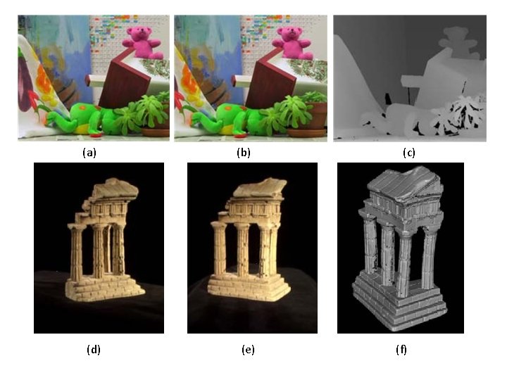
 original color image; (b) ground truth disparities; (c–e) three (x; y) slices for")
")

 • This limitation to sparse correspondences was partially due")

 (d) (b) (e) (c) (f) (g) (a) circular arc fitting in the epipolar")
 • The first step in")

 • It is based on the observation that stereo")
 • For example, the traditional sum-of-squared differences (SSD) algorithm")
 • Local (window-based) algorithms (Section 11. 4), where the")
 • Global algorithms, on the other hand, make explicit")

 • The most common pixel-based matching costs include")
 • Based on binary features such as edges")

 Figure 11. 8 Shiftable window (Scharstein and Szeliski 2002)")
 • Windows with adaptive sizes (Okutomi and Kanade 1992;")
 (a) (b) (c) (d) Figure 11. 9 Aggregation window")
 • Selecting the right window is important, since windows")
 • In local methods, the emphasis is on the")

 • However for image-based rendering, such")
 • Sub-pixel disparity estimates can be")
 • Besides sub-pixel computations, there are")
 (b) (c) Figure 11. 10 Uncertainty in stereo depth estimation (Szeliski 1991 b):")

 • The objective is to find a solution d")
 • The smoothness term is often restricted to measuring")
 • Once the global energy has been defined, a")
 • While global optimization techniques currently produce the best")
 • Cooperative algorithms – Such algorithms iteratively update disparity")

 • Find min-cost path through graph.")
 (b) (c) (d) Figure 11. 12 Segmentation-based stereo")
 (a) Figure 11. 13 Stereo matching with adaptive")

")
 • Foreground objects occlude background objects, which can be")
 • A closely related topic to multi-frame stereo estimation")
 c 2005 IEEE. (Wedel, Rabe, Vaudrey et al.")

 • In order to")

- Slides: 53
Advanced Computer Vision Chapter 11 Stereo Correspondence Presented by: 傅楸善 & 陳弘毅 0922489262 r 4922099@ntu. edu. tw 指導教授: 傅楸善 博士
Introduction • Stereo matching is the process of taking two or more images and estimating a 3 D model of the scene by finding matching pixels in the images and converting their 2 D positions into 3 D depths. • In this chapter, we address the question of how to build a more complete 3 D model.
11. 1 Epipolar Geometry • Given a pixel in one image, how can we compute its correspondence in the other image? • We exploit this information to reduce the number of potential correspondences, and both speed up the matching and increase its reliability.
(Faugeras and Luong 2001; Hartley and Zisserman 2004).
11. 1. 1 Rectification • We can use the epipolar line corresponding to a pixel in one image to constrain the search for corresponding pixels in the other image. • One way to do this is to use a general correspondence algorithm, such as optical flow. • A more efficient algorithm can be obtained by first rectifying (i. e, warping).
(a) (c) (b) (d) (a) Original image pair overlaid with several epipolar lines; (b) images transformed so that epipolar lines are parallel; (c) images rectified so that epipolar lines are horizontal and in vertial correspondence; (d) final rectification that minimizes horizontal distortions. (Loop and Zhang 1999; Faugeras and Luong 2001; Hartley and Zisserman 2004).
11. 1. 1 Rectification (cont’) • The resulting standard rectified geometry is employed in a lot of stereo camera setups and stereo algorithms, and leads to a very simple inverse relationship between 3 D depths Z and disparities d, • where f is the focal length (measured in pixels), B is the baseline, and (Bolles, Baker, and Marimont 1987; Okutomi and Kanade 1993; Scharstein and Szeliski 2002).
11. 1. 1 Rectification (cont’) • The task of extracting depth from a set of images then becomes one of estimating the disparity map d(x, y). • After rectification, we can easily compare the similarity of pixels at corresponding locations (x, y) and (x 0, y 0) = (x + d, y) and store them in a disparity space image C(x, y, d) for further processing
(a) original color image; (b) ground truth disparities; (c–e) three (x; y) slices for d = 10; 16; 21; (f) an (x, d) slice for y = 151 (the dashed line in (b)). Various dark(matching) regions are visible in (c–e), e. g. , the bookshelves, table and cans, and head statue, and three disparity levels can be seen as horizontal lines in (f). The dark bands in the DSIs indicate regions that match at this disparity. (Smaller dark regions are often the result of textureless regions. )
11. 1. 2 Plane sweep Sweeping a set of planes through a scene (a) The set of planes seen from a virtual camera induces a set of homographies in any other source (input) camera image. (b) The warped images from all the other cameras can be stacked into a generalized disparity space volume ~I(x; y; d; k) indexed by pixel location (x; y), disparity d, and camera k.
11. 2 Sparse correspondence • Early stereo matching algorithms were featurebased, i. e. , they first extracted a set of potentially matchable image locations, using either interest operators or edge detectors, and then searched for corresponding locations in other images using a patch-based metric. (Hannah 1974; Marr and Poggio 1979; Mayhew and Frisby 1980; Baker and Binford 1981; Arnold 1983; Grimson 1985; Ohta and Kanade 1985; Bolles, Baker, and Marimont 1987; Matthies, Kanade, and Szeliski 1989; Hsieh, Mc. Keown, and Perlant 1992; Bolles, Baker, and Hannah 1993).
11. 2 Sparse correspondence (cont’) • This limitation to sparse correspondences was partially due to computational resource limitations. • Also driven by a desire to limit the answers produced by stereo algorithms to matches with high certainty. • In some applications, there was also a desire to match scenes with potentially very different illuminations. (Collins 1996).
11. 2. 1 3 D curves and profiles • Another example of sparse correspondence is the matching of profile curves. • Let us assume that the camera is moving smoothly enough that the local epipolar geometry varies slowly.
(a) (d) (b) (e) (c) (f) (g) (a) circular arc fitting in the epipolar plane; (b) synthetic example of an ellipsoid with a truncated side and elliptic surface markings; (c) partially reconstructed surface mesh seen from an oblique and top-down view; (d) real-world image sequence of a soda can on a turntable; (e) extracted edges; (f) partially reconstructed profile curves; (g) partially reconstructed surface mesh.
11. 2. 1 3 D curves and profiles (cont’) • The first step in the processing pipeline is to extract and link edges in each of the input images. • Next, edgels in successive images are matched using pairwise epipolar geometry. (Szeliski and Weiss 1998)
11. 3 Dense correspondence • While sparse matching algorithms are still occasionally used, most stereo matching algorithms today focus on dense correspondence, since this is required for applications such as image-based rendering or modeling. • This problem is more challenging than sparse correspondence.
11. 3 Dense correspondence (cont’) • It is based on the observation that stereo algorithms generally perform some subset of the following four steps: – – 1. matching cost computation; 2. cost (support) aggregation; 3. disparity computation and optimization; and 4. disparity refinement.
11. 3 Dense correspondence (cont’) • For example, the traditional sum-of-squared differences (SSD) algorithm can be described as: – 1. The matching cost is the squared difference of intensity values at a given disparity. – 2. Aggregation is done by summing the matching cost over square windows with constant disparity. – 3. Disparities are computed by selecting the minimal (winning) aggregated value at each pixel.
11. 3 Dense correspondence (cont’) • Local (window-based) algorithms (Section 11. 4), where the disparity computation at a given point depends only on intensity values within a finite window. • Usually make implicit smoothness assumptions by aggregating support.
11. 3 Dense correspondence (cont’) • Global algorithms, on the other hand, make explicit smoothness assumptions and then solve a global optimization problem (Section 11. 5). • Such algorithms typically do not perform an aggregation step, but rather seek a disparity assignment (step 3) that minimizes a global cost function that consists of data (step 1) terms and smoothness terms.
11. 3. 1 Similarity measures • The first component of any dense stereo matching algorithm is a similarity measure that compares pixel values in order to determine how likely they are to be in correspondence. • We briefly review the similarity measures.
11. 3. 1 Similarity measures (cont’) • The most common pixel-based matching costs include sums of squared intensity differences (SSD) (Hannah 1974) • Based on the entropy of the pixel values at a particular disparity hypothesis (Zitnick, Kang, Uyttendaele et al. 2004)
11. 3. 1 Similarity measures (cont’) • Based on binary features such as edges (Baker and Binford 1981; Grimson 1985). • Gradient based measures (Seitz 1989; Scharstein 1994). • The census transform was found by (Hirschm¨uller and Scharstein 2009).
11. 4 Local methods • Local and window-based methods aggregate the matching cost by summing or averaging over a support region in the DSI C(x, y, d). • DSI: Disparity Space Image • Aggregation has been implemented using square windows or Gaussian convolution (traditional). • Shiftable windows (Arnold 1983; Fusiello, Roberto, and Trucco 1997; Bobick and Intille 1999)
11. 4 Local methods (cont’) Figure 11. 8 Shiftable window (Scharstein and Szeliski 2002) c 2002 Springer. The effect of trying all 3 x 3 shifted windows around the black pixel is the same as taking the minimum matching score across all centered (non-shifted) windows in the same neighborhood. (For clarity, only three of the neighboring shifted windows are shown here. )
11. 4 Local methods (cont’) • Windows with adaptive sizes (Okutomi and Kanade 1992; Kanadeand Okutomi 1994; Kang, Szeliski, and Chai 2001; Veksler 2001, 2003). • Results of color-based segmentation (Yoon and Kweon 2006; Tombari, Mattoccia, Di Stefano et al. 2008).
11. 4 Local methods (cont’) (a) (b) (c) (d) Figure 11. 9 Aggregation window sizes and weights adapted to image content (Tombari, Mattoccia, Di Stefano et al. 2008) c 2008 IEEE: (a) original image with selected evaluation points; (b) variable windows (Veksler 2003); (c) adaptive weights (Yoon and Kweon 2006); (d) segmentation-based (Tombari, Mattoccia, and Di Stefano 2007). Notice how the adaptive weights and segmentation-based techniques adapt their support to similarly colored pixels.
11. 4 Local methods (cont’) • Selecting the right window is important, since windows must be large enough to contain sufficient texture and yet small enough so that they do not straddle depth discontinuities. • An alternative method for aggregation is iterative diffusion, i. e. , repeatedly adding to each pixel’s cost the weighted values of its neighboring pixels’ costs (Szeliski and Hinton 1985; Shah 1993; Scharstein and Szeliski 1998).
11. 4 Local methods (cont’) • In local methods, the emphasis is on the matching cost computation and cost aggregation steps. • Computing the final disparities is trivial: simply choose at each pixel the disparity associated with the minimum cost value.
11. 4. 1 Sub-pixel estimation and uncertainty • Most stereo correspondence algorithms compute a set of disparity estimates in some discretized space, e. g. , for integer disparities. • For applications such as robot navigation or people tracking, these may be perfectly adequate.
11. 4. 1 Sub-pixel estimation and uncertainty (cont’) • However for image-based rendering, such quantized maps lead to very unappealing view synthesis results. • To remedy this situation, many algorithms apply a sub-pixel refinement stage after the initial discrete correspondence stage.
11. 4. 1 Sub-pixel estimation and uncertainty (cont’) • Sub-pixel disparity estimates can be computed in a variety of ways, including iterative gradient descent and fitting a curve to the matching costs at discrete disparity levels.
11. 4. 1 Sub-pixel estimation and uncertainty (cont’) • Besides sub-pixel computations, there are other ways of post-processing the computed disparities. • Associate confidences with per-pixel depth estimates, which can be done by looking at the curvature of the correlation surface.
(a) (b) (c) Figure 11. 10 Uncertainty in stereo depth estimation (Szeliski 1991 b): (a) input image; (b) estimated depth map (blue is closer); (c) estimated confidence(red is higher). As you can see, more textured areas have higher confidence.
11. 5 Global optimization • Global stereo matching methods perform some optimization or iteration steps after the disparity computation phase and often skip the aggregation step altogether. • Many global methods are formulated in an energyminimization framework.
11. 5 Global optimization (cont’) • The objective is to find a solution d that minimizes a global energy, • The data term, Ed(d), measures how well the disparity function d agrees with the input image pair. • where C is the (initial or aggregated) matching cost DSI.
11. 5 Global optimization (cont’) • The smoothness term is often restricted to measuring only the differences between neighboring pixels’ disparities, where ᵨ is some monotonically increasing function of disparity difference.
11. 5 Global optimization (cont’) • Once the global energy has been defined, a variety of algorithms can be used to find a (local) minimum. • Traditional approaches associated with regularization and Markov random fields include continuation (Blake and Zisserman 1987)
11. 5 Global optimization (cont’) • While global optimization techniques currently produce the best stereo matching results, there are some alternative approaches worth studying. – Cooperative algorithms. – Coarse-to-fine and incremental warping.
11. 5 Global optimization (cont’) • Cooperative algorithms – Such algorithms iteratively update disparity estimates using non-linear operations that result in an overall behavior similar to global optimization algorithms. (Dev 1974; Marr and Poggio 1976; Marroquin 1983; Szeliski and Hinton 1985; Zitnick and Kanade 2000). • Coarse-to-fine and incremental warping – Here, images are successively warped and disparity estimates incrementally updated until a satisfactory registration is achieved. (Quam 1984; Bergen, Anandan, Hanna et al. 1992; Barron, Fleet, and Beauchemin 1994; Szeliski and Coughlan 1997).
11. 5. 1 Dynamic programming • Treat feature correspondence as graph problem.
11. 5. 1 Dynamic programming (cont’) • Find min-cost path through graph.
11. 5. 2 Segmentation-based techniques (a) (b) (c) (d) Figure 11. 12 Segmentation-based stereo matching (Zitnick, Kang, Uyttendaele et al. 2004) © 2004 ACM: (a) input color image; (b) color-based segmentation; (c) initial disparity estimates; (d) final piecewise-smoothed disparities.
11. 5. 2 Segmentation-based techniques (cont’) (a) Figure 11. 13 Stereo matching with adaptive over-segmentation and matting (Taguchi, Wilburn, and Zitnick 2008) c 2008 IEEE: (a) segment boundaries are refined during the optimization, leading to more accurate results (e. g. , the thin green leaf in the bottom row);
11. 6 Multi-view stereo • While matching pairs of images is a useful way of obtaining depth information, matching more images can lead to even better results. • A useful way to visualize the multi-frame stereo estimation problem is to examine the epipolar plane image (EPI) formed by stacking corresponding scanlines from all the images.
11. 6 Multi-view stereo (cont’)
11. 6 Multi-view stereo (cont’) • Foreground objects occlude background objects, which can be seen as occluding other strips in the EPI. • If we are given a dense enough set of images, we can find such strips and reason about their relationships in order to both reconstruct the 3 D scene and make inferences about translucent and specular reflections.
11. 6 Multi-view stereo (cont’) • A closely related topic to multi-frame stereo estimation is scene flow. • Multiple cameras are used to capture a dynamic scene. • The task is then to simultaneously recover the 3 D shape of the object at every instant in time.
(Vedula, Baker, Rander et al. 2005) c 2005 IEEE. (Wedel, Rabe, Vaudrey et al. 2008) c 2008 Springer.
11. 6. 1 Volumetric and 3 D surface reconstruction
11. 6. 1 Volumetric and 3 D surface reconstruction (cont’) • In order to organize and compare all these techniques, Seitz, Curless, Diebel et al. (2006)developed a six-point taxonomy that can help classify algorithms according to the – – – scene representation photoconsistency measure visibility model shape priors reconstruction algorithm initialization requirements • For more details, please consult the full survey paper (Seitz, Curless, Diebel et al. 2006) and the evaluation Web site, http: //vision. middlebury. edu/mview/
X