Advanced Computer Programming Scipy Module Sinan AYDIN What

What is Scipy? Scipy Module The scipy package contains various toolboxes dedicated different submodules

File input/output: scipy. io Scipy Module Sci. Py has many modules, classes, and functions

Linear algebra operations: scipy. linalg Scipy Module import numpy as np from scipy import

Optimization and fit: scipy. optimize Optimization is the problem of ﬁnding a numerical solution

Optimization and fit: scipy. optimize Exercise: Curve ﬁtting of temperature data The temperature extremes

Optimization and fit: scipy. optimize Scipy Module Exercise: Curve ﬁtting of temperature data The

Statistics and random numbers: scipy. stats Scipy Module The module scipy. statscontains statistical tools

Statistics and random numbers: numpy Scipy Module Mean, median and percentiles import numpy as

Statistical tests: scipy. stats Scipy Module A statistical test is a decision indicator. For

Statistical tests: scipy. stats Scipy Module https: //docs. scipy. org/doc/scipy/reference/stats. html

Numerical integration: scipy. integrate Scipy Module Function integrals from scipy import integrate import numpy

Image manipulation: scipy. ndimage Scipy Module The misc package in Sci. Py comes with

Slides: 15

Download presentation

Advanced Computer Programming Scipy Module Sinan AYDIN

What is Scipy? Scipy Module The scipy package contains various toolboxes dedicated different submodules correspond to different applications image processing, statistics, special functions, etc. Scipyis composed of task-speciﬁc sub-modules: https: //docs. scipy. org/doc/scipy/reference/p y-modindex. html

File input/output: scipy. io Scipy Module Sci. Py has many modules, classes, and functions available to read data from and write data to a variety of file formats. MATLAB® files import numpy as np from scipy import io as spio a = np. ones((3, 3)) b = np. zeros((5, 5)) spio. savemat('file. mat', {'a': a, 'b': b}) # savemat expects a dictionary data = spio. loadmat('file. mat') print(data['a']) print(data['b']) IDL® files Wav sound files (scipy. io. wavfile) Matrix Market files Arff files (scipy. io. arff) Unformatted Fortran files Netcdf Harwell-Boeing files https: //docs. scipy. org/doc/scipy/reference/io. html#module-scipy. io

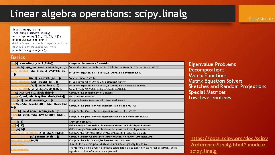
Linear algebra operations: scipy. linalg Scipy Module import numpy as np from scipy import linalg arr = np. array([[1, 2], [3, 4]]) print(linalg. det(arr)) #Value. Error: expected square matrix #linalg. det(np. ones((3, 4))) print(linalg. inv(arr)) Basics inv(a[, overwrite_a, check_finite]) solve(a, b[, sym_pos, lower, overwrite_a, …]) solve_banded(l_and_u, ab, b[, overwrite_ab, …]) solveh_banded(ab, b[, overwrite_ab, …]) solve_circulant(c, b[, singular, tol, …]) solve_triangular(a, b[, trans, lower, …]) solve_toeplitz(c_or_cr, b[, check_finite]) det(a[, overwrite_a, check_finite]) norm(a[, ord, axis, keepdims, check_finite]) lstsq(a, b[, cond, overwrite_a, …]) pinv(a[, cond, return_rank, check_fini te]) pinv 2(a[, cond, return_rank, …]) pinvh(a[, cond, rcond, lower, return_rank, … ]) kron(a, b) tril(m[, k]) triu(m[, k]) orthogonal_procrustes(A, B[, check_finite]) matrix_balance(A[, permute, scale, …]) subspace_angles(A, B) Lin. Alg. Error Lin. Alg. Warning Compute the inverse of a matrix. Solves the linear equation set a * x = b for the unknown x for square a matrix. Solve the equation a x = b for x, assuming a is banded matrix. Solve equation a x = b. Solve C x = b for x, where C is a circulant matrix. Solve the equation a x = b for x, assuming a is a triangular matrix. Solve a Toeplitz system using Levinson Recursion Compute the determinant of a matrix Matrix or vector norm. Compute least-squares solution to equation Ax = b. Eigenvalue Problems Decompositions Matrix Functions Matrix Equation Solvers Sketches and Random Projections Special Matrices Low-level routines Compute the (Moore-Penrose) pseudo-inverse of a matrix. Compute the (Moore-Penrose) pseudo-inverse of a Hermitian matrix. Kronecker product. Make a copy of a matrix with elements above the k-th diagonal zeroed. Make a copy of a matrix with elements below the k-th diagonal zeroed. Compute the matrix solution of the orthogonal Procrustes problem. Compute a diagonal similarity transformation for row/column balancing. Compute the subspace angles between two matrices. Generic Python-exception-derived object raised by linalg functions. The warning emitted when a linear algebra related operation is close to fail conditions of the algorithm or loss of accuracy is expected. https: //docs. scipy. org/doc/scipy /reference/linalg. html# modulescipy. linalg

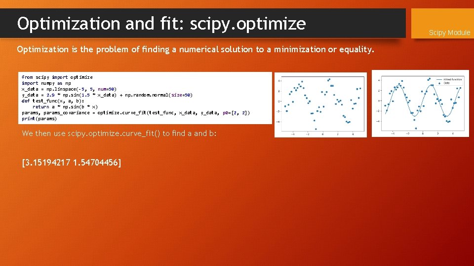
Optimization and fit: scipy. optimize Optimization is the problem of ﬁnding a numerical solution to a minimization or equality. from scipy import optimize import numpy as np x_data = np. linspace(-5, 5, num=50) y_data = 2. 9 * np. sin(1. 5 * x_data) + np. random. normal(size=50) def test_func(x, a, b): return a * np. sin(b * x) params, params_covariance = optimize. curve_fit(test_func, x_data, y_data, p 0=[2, 2]) print(params) We then use scipy. optimize. curve_fit() to ﬁnd a and b: [3. 15194217 1. 54704456] Scipy Module

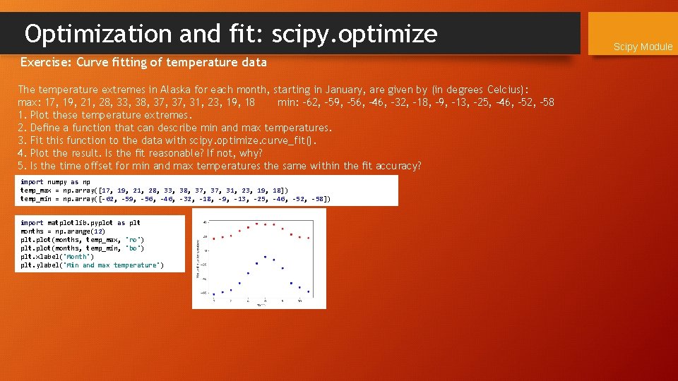
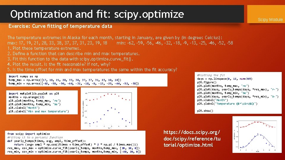
Optimization and fit: scipy. optimize Exercise: Curve fitting of temperature data The temperature extremes in Alaska for each month, starting in January, are given by (in degrees Celcius): max: 17, 19, 21, 28, 33, 38, 37, 31, 23, 19, 18 min: -62, -59, -56, -46, -32, -18, -9, -13, -25, -46, -52, -58 1. Plot these temperature extremes. 2. Define a function that can describe min and max temperatures. 3. Fit this function to the data with scipy. optimize. curve_fit(). 4. Plot the result. Is the fit reasonable? If not, why? 5. Is the time offset for min and max temperatures the same within the fit accuracy? import numpy as np temp_max = np. array([17, 19, 21, 28, 33, 38, 37, 31, 23, 19, 18]) temp_min = np. array([-62, -59, -56, -46, -32, -18, -9, -13, -25, -46, -52, -58]) import matplotlib. pyplot as plt months = np. arange(12) plt. plot(months, temp_max, 'ro') plt. plot(months, temp_min, 'bo') plt. xlabel('Month') plt. ylabel('Min and max temperature') Scipy Module

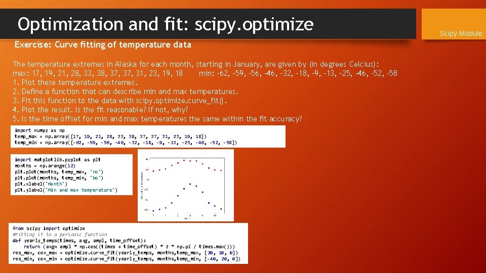
Optimization and fit: scipy. optimize Scipy Module Exercise: Curve fitting of temperature data The temperature extremes in Alaska for each month, starting in January, are given by (in degrees Celcius): max: 17, 19, 21, 28, 33, 38, 37, 31, 23, 19, 18 min: -62, -59, -56, -46, -32, -18, -9, -13, -25, -46, -52, -58 1. Plot these temperature extremes. 2. Define a function that can describe min and max temperatures. 3. Fit this function to the data with scipy. optimize. curve_fit(). 4. Plot the result. Is the fit reasonable? If not, why? 5. Is the time offset for min and max temperatures the same within the fit accuracy? import numpy as np temp_max = np. array([17, 19, 21, 28, 33, 38, 37, 31, 23, 19, 18]) temp_min = np. array([-62, -59, -56, -46, -32, -18, -9, -13, -25, -46, -52, -58]) import matplotlib. pyplot as plt months = np. arange(12) plt. plot(months, temp_max, 'ro') plt. plot(months, temp_min, 'bo') plt. xlabel('Month') plt. ylabel('Min and max temperature') from scipy import optimize #Fitting it to a periodic function def yearly_temps(times, avg, ampl, time_offset): return (avg+ ampl * np. cos((times + time_offset) * 2 * np. pi / times. max())) res_max, cov_max = optimize. curve_fit(yearly_temps, months, temp_max, [20, 10, 0]) res_min, cov_min = optimize. curve_fit(yearly_temps, months, temp_min, [-40, 20, 0]) #Plotting the fit days = np. linspace(0, 12, num=365) plt. figure() plt. plot(months, temp_max, 'ro') plt. plot(days, yearly_temps(days, *res_max), 'r-') plt. plot(months, temp_min, 'bo') plt. plot(days, yearly_temps(days, *res_min), 'b-') plt. xlabel('Month') plt. ylabel('Temperature ($^circ$C)') plt. show() https: //docs. scipy. org/ doc/scipy/reference/tu torial/optimize. html

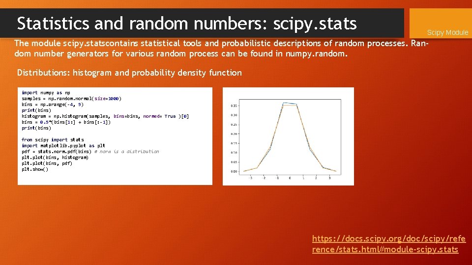
Statistics and random numbers: scipy. stats Scipy Module The module scipy. statscontains statistical tools and probabilistic descriptions of random processes. Random number generators for various random process can be found in numpy. random. Distributions: histogram and probability density function import numpy as np samples = np. random. normal(size=1000) bins = np. arange(-4, 5) print(bins) histogram = np. histogram(samples, bins=bins, normed= True )[0] bins = 0. 5*(bins[1: ] + bins[: -1]) print(bins) from scipy import stats import matplotlib. pyplot as plt pdf = stats. norm. pdf(bins) # norm is a distribution plt. plot(bins, histogram) plt. plot(bins, pdf) plt. show() https: //docs. scipy. org/doc/scipy/refe rence/stats. html#module-scipy. stats

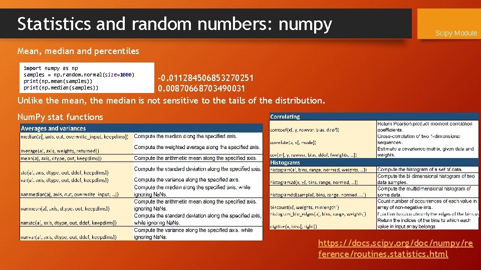
Statistics and random numbers: numpy Scipy Module Mean, median and percentiles import numpy as np samples = np. random. normal(size=1000) print(np. mean(samples)) print(np. median(samples)) -0. 011284506853270251 0. 00870668703490031 Unlike the mean, the median is not sensitive to the tails of the distribution. Num. Py stat functions https: //docs. scipy. org/doc/numpy/re ference/routines. statistics. html

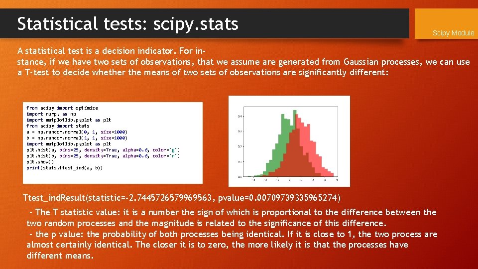
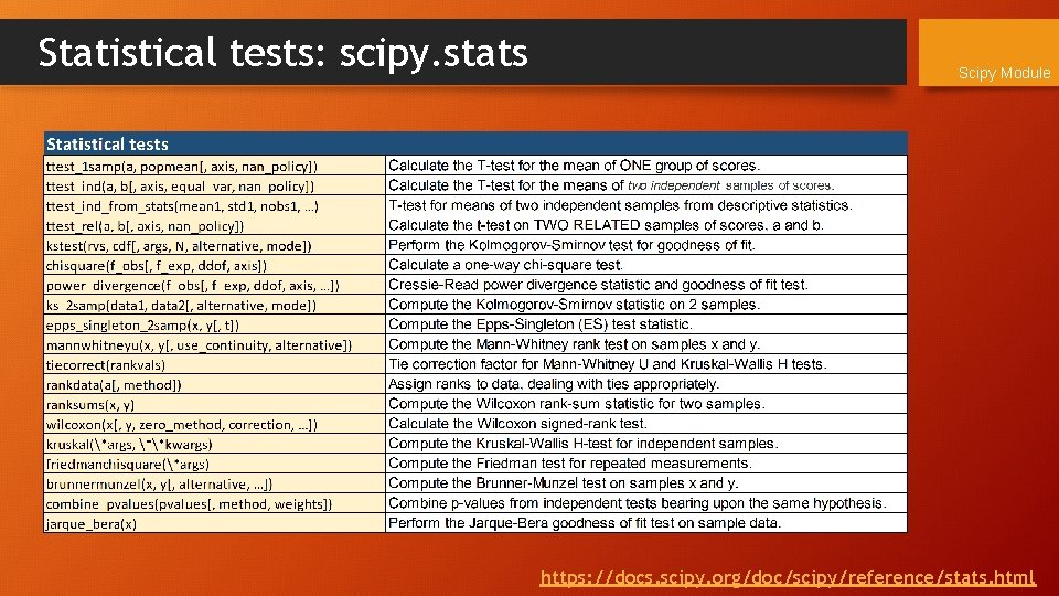
Statistical tests: scipy. stats Scipy Module A statistical test is a decision indicator. For instance, if we have two sets of observations, that we assume are generated from Gaussian processes, we can use a T-test to decide whether the means of two sets of observations are signiﬁcantly different: from scipy import optimize import numpy as np import matplotlib. pyplot as plt from scipy import stats a = np. random. normal(0, 1, size=1000) b = np. random. normal(1, 1, size=1000) import matplotlib. pyplot as plt. hist(a, bins=25, density=True, alpha=0. 6, color='g') plt. hist(b, bins=25, density=True, alpha=0. 6, color='r') plt. show() print(stats. ttest_ind(a, b)) Ttest_ind. Result(statistic=-2. 7445726579969563, pvalue=0. 00709739335965274) - The T statistic value: it is a number the sign of which is proportional to the difference between the two random processes and the magnitude is related to the signiﬁcance of this difference. - the p value: the probability of both processes being identical. If it is close to 1, the two process are almost certainly identical. The closer it is to zero, the more likely it is that the processes have different means.

Statistical tests: scipy. stats Scipy Module https: //docs. scipy. org/doc/scipy/reference/stats. html

Numerical integration: scipy. integrate Scipy Module Function integrals from scipy import integrate import numpy as np res, err = integrate. quad(np. sin, 0, np. pi/2) print("quad Function result and err") print(res, err) # res is the result, err is an estimate of the err print("quadrature function result ") print( "integral of sin (0, pi/2") print(integrate. quadrature(np. cos, 0. 0, np. pi/2)) print( "# analytical result") print(np. sin(np. pi/2)-np. sin(0)) # analytical result print( "romberg function steps and result (0, pi/2)") result=integrate. romberg(np. cos, 0. 0, np. pi/2, show=True) print(result) quad Function result and err 0. 99999999 1. 1102230246251564 e-14 quadrature function result integral of sin (0, pi/2 (0. 9999999536, 3. 9611425250996035 e-11) # analytical result 1. 0 romberg function steps and result (0, pi/2) Romberg integration of <function vectorize 1. <locals>. vfunc at 0 x 02 CF 07 C 8> from [0. 0, 1. 5707963267948966] Steps 1 2 4 8 16 Step. Size 1. 570796 0. 785398 0. 392699 0. 196350 0. 098175 Results 0. 785398 0. 948059 0. 987116 0. 996785 0. 999197 1. 002280 1. 000135 1. 000008 1. 000001 0. 999992 1. 000000 The final result is 0. 99999980171 after 17 function evaluations. 0. 99999980171 https: //docs. scipy. org/doc/scipy/reference/integrate. html#integration-and-odes-scipy-integrate

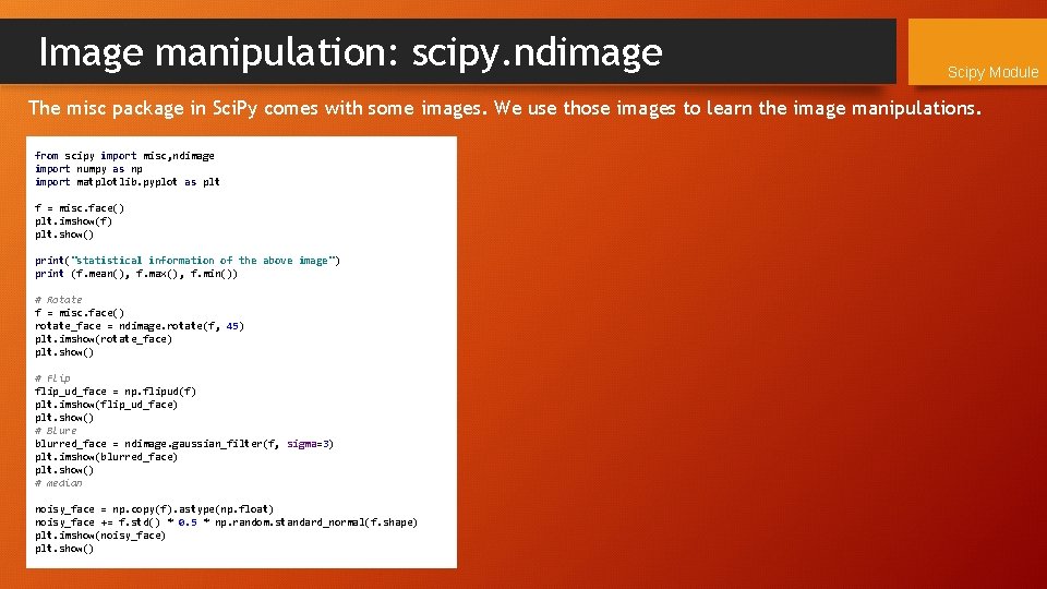
Image manipulation: scipy. ndimage Scipy Module The misc package in Sci. Py comes with some images. We use those images to learn the image manipulations. from scipy import misc, ndimage import numpy as np import matplotlib. pyplot as plt f = misc. face() plt. imshow(f) plt. show() print("statistical information of the above image") print (f. mean(), f. max(), f. min()) # Rotate f = misc. face() rotate_face = ndimage. rotate(f, 45) plt. imshow(rotate_face) plt. show() # Flip flip_ud_face = np. flipud(f) plt. imshow(flip_ud_face) plt. show() # Blure blurred_face = ndimage. gaussian_filter(f, sigma=3) plt. imshow(blurred_face) plt. show() # median noisy_face = np. copy(f). astype(np. float) noisy_face += f. std() * 0. 5 * np. random. standard_normal(f. shape) plt. imshow(noisy_face) plt. show()