Advanced Computer Graphics CSE 163 Spring 2017 Lecture

Advanced Computer Graphics CSE 163 [Spring 2017], Lecture 2 Ravi Ramamoorthi http: //www. cs. ucsd. edu/~ravir

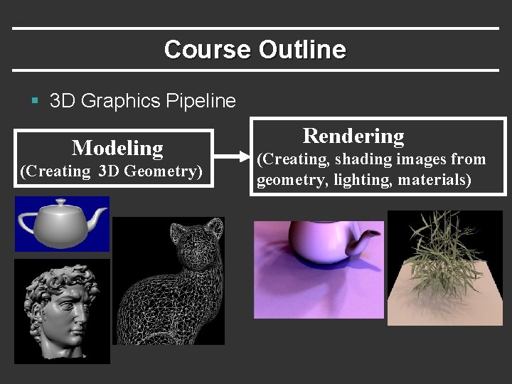
Course Outline § 3 D Graphics Pipeline Modeling (Creating 3 D Geometry) Rendering (Creating, shading images from geometry, lighting, materials)

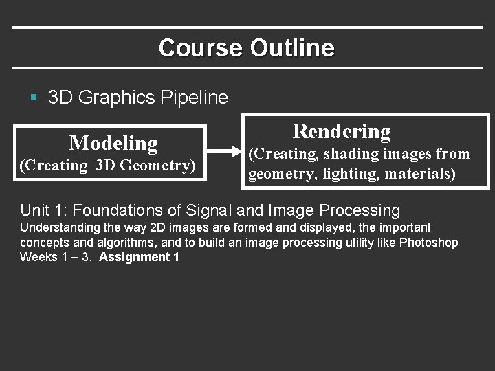
Course Outline § 3 D Graphics Pipeline Modeling (Creating 3 D Geometry) Rendering (Creating, shading images from geometry, lighting, materials) Unit 1: Foundations of Signal and Image Processing Understanding the way 2 D images are formed and displayed, the important concepts and algorithms, and to build an image processing utility like Photoshop Weeks 1 – 3. Assignment 1

To Do § Assignment 1, Due Apr 28. § § § Anyone need help finding partners? Should already have downloaded code, skimmed assn After today, enough to finish 3. 2, 3. 3 (first half) Should START EARLY (this week) on assn Second half next week. § Class participation, discussion important § If you have to miss a class, see podcast if available § Please sign up for Piazza

Outline § Intensity and Color (briefly) § Basic operations (3. 2 in assignment [10 points]) § Quantization, Halftoning and Dithering § (3. 3 in assignment [10 points]) § Next week: Sampling and Reconstruction § Including signal processing and fourier analysis § Implementation of simple digital filters, resizing § Second half of assignment § Lectures main source; will also try handout

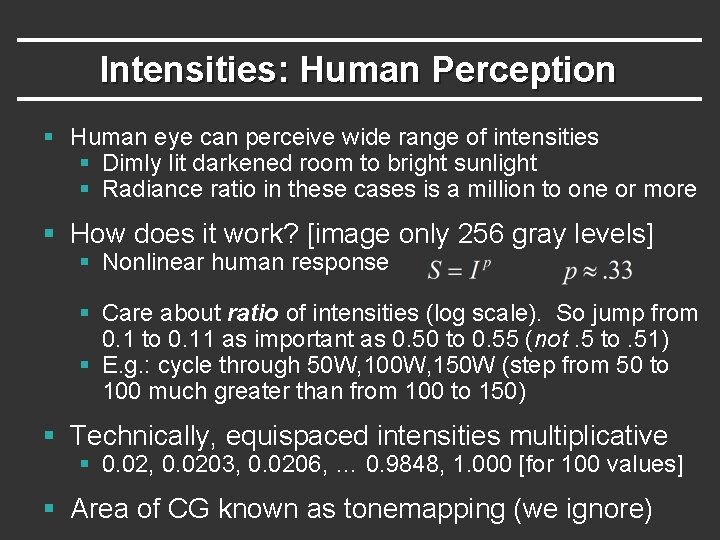
Intensities: Human Perception § Human eye can perceive wide range of intensities § Dimly lit darkened room to bright sunlight § Radiance ratio in these cases is a million to one or more § How does it work? [image only 256 gray levels] § Nonlinear human response § Care about ratio of intensities (log scale). So jump from 0. 1 to 0. 11 as important as 0. 50 to 0. 55 (not. 5 to. 51) § E. g. : cycle through 50 W, 100 W, 150 W (step from 50 to 100 much greater than from 100 to 150) § Technically, equispaced intensities multiplicative § 0. 02, 0. 0203, 0. 0206, … 0. 9848, 1. 000 [for 100 values] § Area of CG known as tonemapping (we ignore)

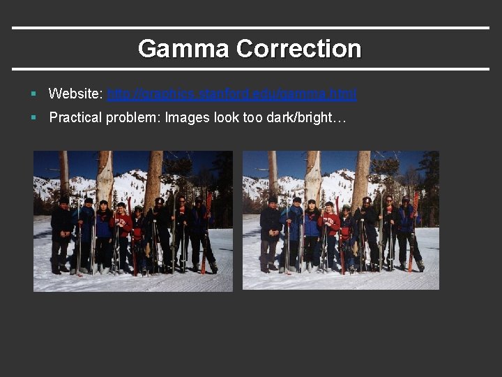
Gamma Correction § Website: http: //graphics. stanford. edu/gamma. html § Practical problem: Images look too dark/bright…

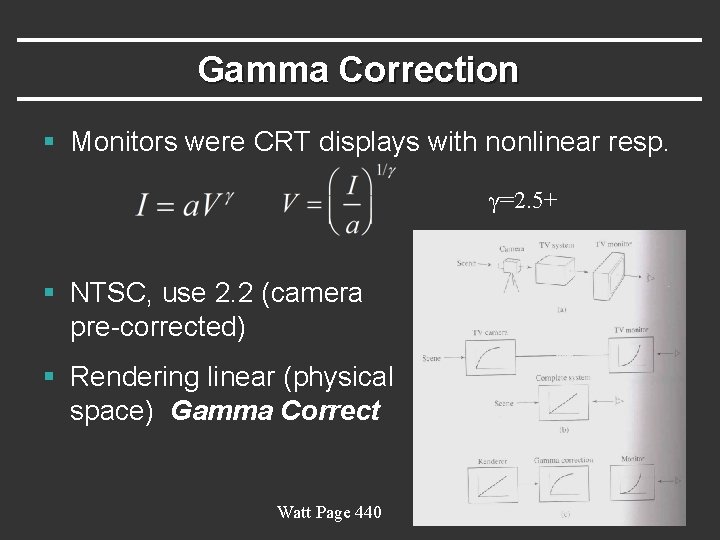
Gamma Correction § Monitors were CRT displays with nonlinear resp. γ=2. 5+ § NTSC, use 2. 2 (camera pre-corrected) § Rendering linear (physical space) Gamma Correct Watt Page 440

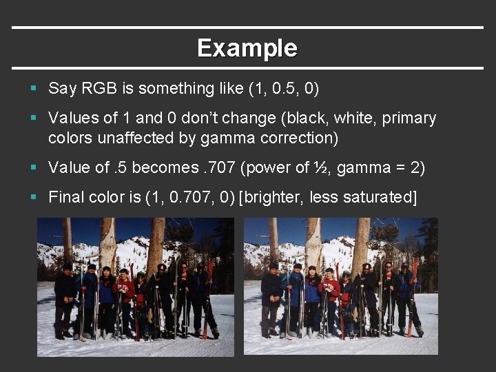
Example § Say RGB is something like (1, 0. 5, 0) § Values of 1 and 0 don’t change (black, white, primary colors unaffected by gamma correction) § Value of. 5 becomes. 707 (power of ½, gamma = 2) § Final color is (1, 0. 707, 0) [brighter, less saturated]

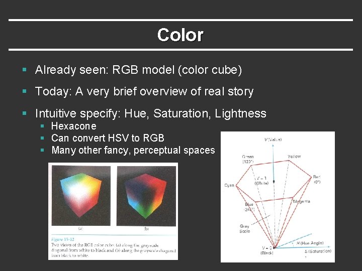
Color § Already seen: RGB model (color cube) § Today: A very brief overview of real story § Intuitive specify: Hue, Saturation, Lightness § Hexacone § Can convert HSV to RGB § Many other fancy, perceptual spaces

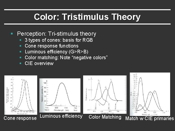
Color: Tristimulus Theory § Perception: Tri-stimulus theory § § § 3 types of cones: basis for RGB Cone response functions Luminous efficiency (G>R>B) Color matching: Note “negative colors” CIE overview Cone response Luminous efficiency Color Matching Match w CIE primaries

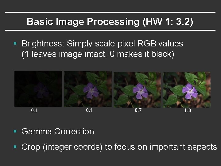
Basic Image Processing (HW 1: 3. 2) § Brightness: Simply scale pixel RGB values (1 leaves image intact, 0 makes it black) 0. 1 0. 4 0. 7 1. 0 § Gamma Correction § Crop (integer coords) to focus on important aspects

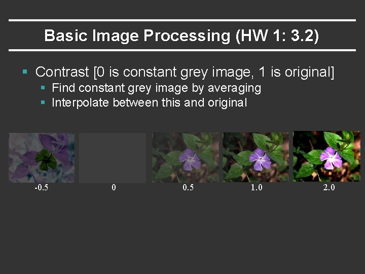
Basic Image Processing (HW 1: 3. 2) § Contrast [0 is constant grey image, 1 is original] § Find constant grey image by averaging § Interpolate between this and original -0. 5 0 0. 5 1. 0 2. 0

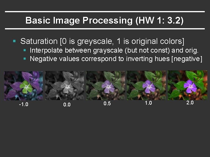
Basic Image Processing (HW 1: 3. 2) § Saturation [0 is greyscale, 1 is original colors] § Interpolate between grayscale (but not const) and orig. § Negative values correspond to inverting hues [negative] -1. 0 0. 5 1. 0 2. 0

Outline § Intensity and Color (briefly) § Basic operations (3. 2 in assignment [10 points] § Quantization, Halftoning and Dithering § (3. 3 in assignment [10 points]) § Next week: Sampling and Reconstruction § Including signal processing and fourier analysis § Implementation of simple digital filters, resizing § Second half of assignment (and written part)

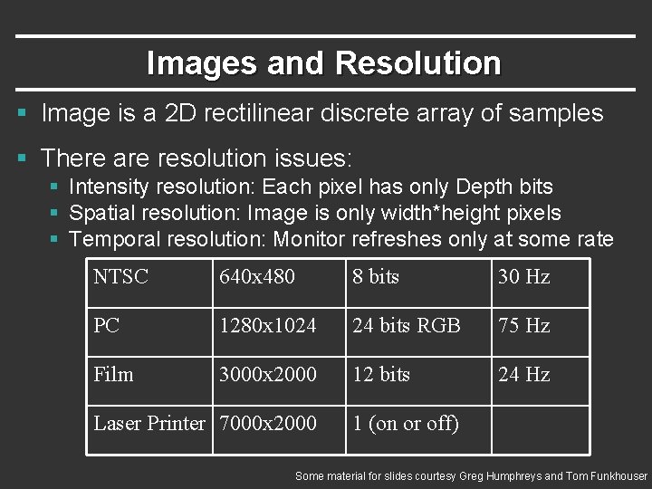
Images and Resolution § Image is a 2 D rectilinear discrete array of samples § There are resolution issues: § Intensity resolution: Each pixel has only Depth bits § Spatial resolution: Image is only width*height pixels § Temporal resolution: Monitor refreshes only at some rate NTSC 640 x 480 8 bits 30 Hz PC 1280 x 1024 24 bits RGB 75 Hz Film 3000 x 2000 12 bits 24 Hz Laser Printer 7000 x 2000 1 (on or off) Some material for slides courtesy Greg Humphreys and Tom Funkhouser

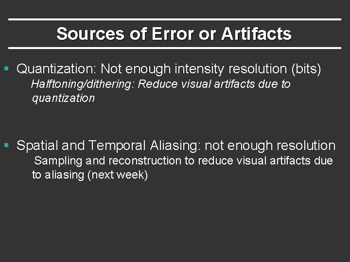
Sources of Error or Artifacts § Quantization: Not enough intensity resolution (bits) Halftoning/dithering: Reduce visual artifacts due to quantization § Spatial and Temporal Aliasing: not enough resolution Sampling and reconstruction to reduce visual artifacts due to aliasing (next week)

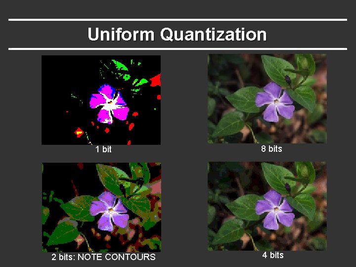
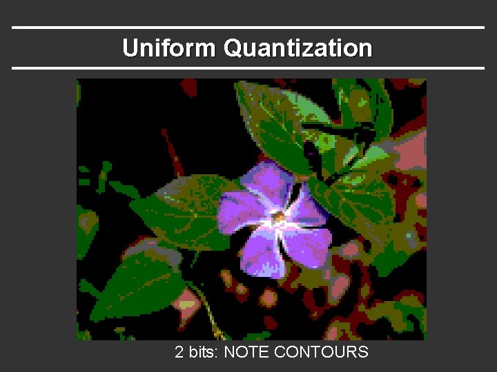
Uniform Quantization 1 bit 8 bits 2 bits: NOTE CONTOURS 4 bits

Uniform Quantization 2 bits: NOTE CONTOURS

Reducing Quantization § Halftoning § Dithering § Random Dither § Error Diffusion (Floyd-Steinberg)

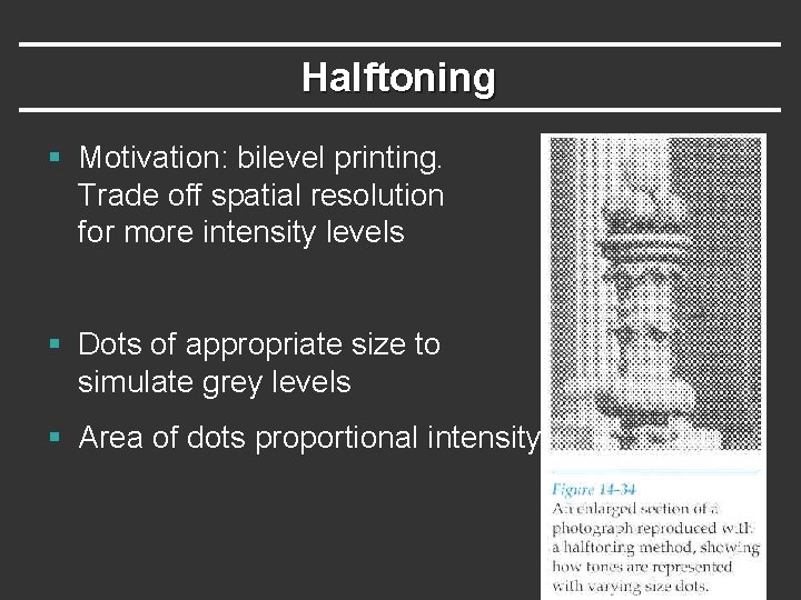
Halftoning § Motivation: bilevel printing. Trade off spatial resolution for more intensity levels § Dots of appropriate size to simulate grey levels § Area of dots proportional intensity

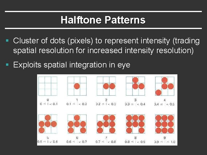
Halftone Patterns § Cluster of dots (pixels) to represent intensity (trading spatial resolution for increased intensity resolution) § Exploits spatial integration in eye

Reducing Quantization § Halftoning § Dithering (distribute errors among pixels) § Random Dither § Error Diffusion (Floyd-Steinberg)

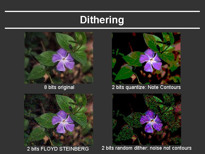
Dithering 8 bits original 2 bits quantize: Note Contours 2 bits FLOYD STEINBERG 2 bits random dither: noise not contours

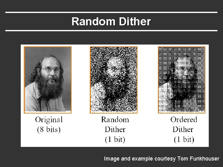
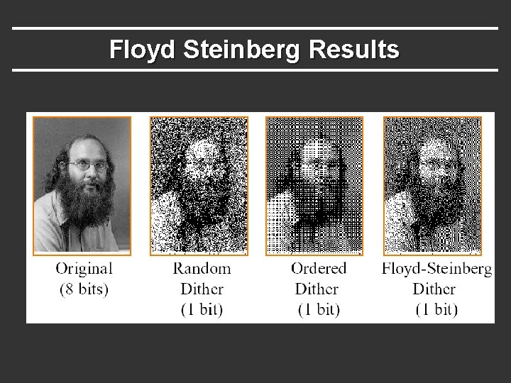
Random Dither § Randomize quantization errors [see assignment for exact details on adding random noise] § Seems silly (add random noise), but eye more tolerant of high-frequency noise than contours or aliasing § More complex algorithms (not considered here) are ordered dither with patterns of thresholds rather than completely random noise

Random Dither Image and example courtesy Tom Funkhouser

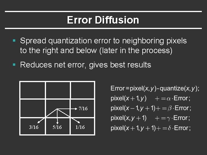
Error Diffusion § Spread quantization error to neighboring pixels to the right and below (later in the process) § Reduces net error, gives best results 7/16 3/16 5/16 1/16

Floyd Steinberg Results

Quantization (Sec 3. 3 Ass 1) § Simple quantization (should be straightforward) § Random Dither (just add noise, pretty simple) § Floyd-Steinberg (trickiest) § Must implement a diffusion of error to other pixels (simply add in appropriate error to them) § Uses fractions, so must use floating point § And possibly negative numbers since error can be minus § Boundary conditions (what if no right etc. ) toroidal [may not be relevant in this case] or change weights appropriately, but don’t darken boundaries