Advanced Applications Support Group Mark Straka National Center

Advanced Applications Support Group Mark Straka National Center for Supercomputing Applications University of Illinois at Urbana-Champaign

The Load Balancing Challenge in Microphysics • Small % of MPI tasks develop serious work • Microphysics can be 20 -30% of simulation time, grows rapidly during cloud formation • Challenge: Gather the points with “work” on busy nodes, share with others, reassemble • Will communication overhead defeat the purpose? • Earlier back-of-envelope calculations indicated marginal potential for balancing speedup, dependent upon network params.

Next slide: MPE graphical depiction of load imbalance • Courtesy Leigh Orf, Central Michigan University • 256 procs, SGI Altix • Microphysics is green areas

Prototype load-balancing code tested on: George Bryan’s CM 1 (r 15) code driving the LFO 3 -ICE MODEL VERSION: 1. 3 with Rates (2/10/05) LIN-FARLEY-ORVILLE-like "Simple Ice and Liquid Microphysics Scheme" based on Gilmore et al. (2004) Mon. Wea. Rev. Copyright (C) <2004> <Jerry Straka and Matthew Gilmore> Gilmore M. S. , J. M. Straka, and E. N. Rasmussen, Monthly Weather Review: Vol. 132, No. 8, pp. 1897 -1916.

LFO balancing scheme • 3 -D “gather” of all ice points to compressed 1 D arrays • Need to send 21 arrays, receive 12 back • Necessary synch points at receivers (front end and back end of routine) • Packing of “send” arrays is not balanceable because it necessarily only happens on heavy nodes, and must precede work sharing

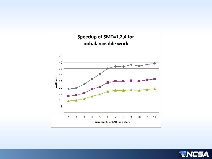
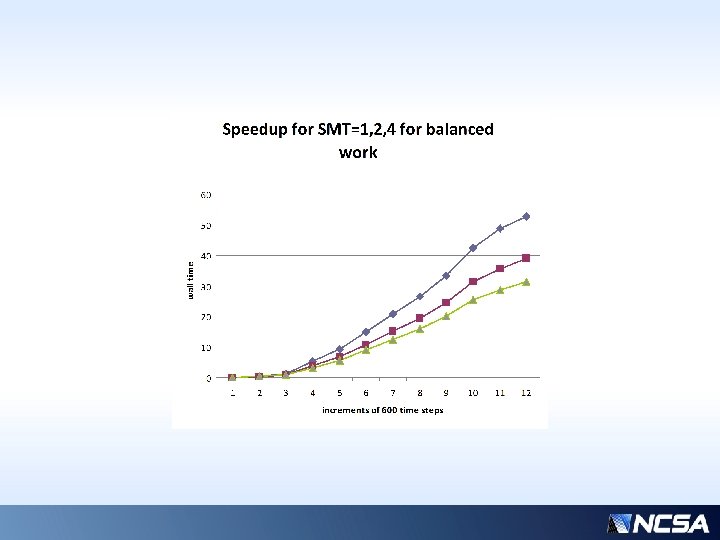
LFO ICE prototype, SMT/OMP • Open. MP constructs have been added to take advantage of SMT (Simultaneous Multi Threading) technology • SMT Allows hybrid model to achieve speedup “for free” since the OMP threads are coscheduled with no additional hardware resources • Of course, hybrid OMP will also work on actual cores, shared with MPI on a node • Some interesting cache effects observed by combining load balancing with OMP…

Simultaneous Multi-Threading (SMT) • Exploits cache misses (instruction and/or data) and/or instruction dependency delays to utilize vacant pipeline slots for execution • Enables the concurrent execution of multiple threads’ instruction streams on the same core • Instruction mixes (and hence pipe utilization) can vary widely during execution • Need to look at SMT as an average improvement for throughput, typically in range of 1. 5 -2 x out of 4. • E. g. POWER 7 has 2 pipes for load/store, 2 pipes for arithmetic, and 1 pipe for branch instructions

Variables Affecting Payoff of Balancing • Number of vertical layers • Total number of processors and network (relative core speed to network) • SMT/OMP interaction with MPI balancing decomposition (local cache effects, loop size) to a lesser degree • Actual fraction of heavy nodes and average distribution of work, evolving over time

Algorithm • Every ~100 time steps, globally share “count” of each processor’s work (i. e. compressed work points) • Found that isends/irecvs somewhat better than collective allgather for this • Find max/min/ave counts and locations among the global data • Iterate, for each max-min pair, send minimum amount necessary required to bring one to the average value.

Algorithm (cont. ) • Iteration process – • Tunable for number of allowable messages, to control granularity (precision) of the balancing • Create send/receive lists and counts • Send and receive according to the pattern of processors determined at the global steps • Allow feedback at intermediate (non-global) steps so that the sender can readjust the target average and redistribute his most current work value to his receivers accordingly

Algorithm (cont. ) • Feedback involves each receiver returning his most current (native) work value to his sender • This compensates for new work which may bubble up during intermediate steps that was not caught by the global steps • Global steps are expensive, so much more efficient to use feedback and readjust amounts of work sent, even though the actual communication pattern does not change (until possibly the next global sharing)

Algorithm (cont. ) • Use of MPI_PROBE to check for variable message sizes allows receivers to adjust to varying workload • Receives/waits are staggered but it really doesn’t matter since nearly all of the wait time will be spent waiting for the first array(s) (e. g. theta 0 or pres 0) which are needed very early in the calculations and thus cannot be hidden effectively

Algorithm (cont. ) • Subgroups of senders/receivers can technically be split into disjoint MPI communicators, but since there is a synchronization at every time step anyway, I decided this was not worth the added complication to the code. • Patterns of senders/receivers are fixed during intermediate steps – reshuffling can occur at the global steps as the max/min distribution evolves • Technically, a static processor distribution could be determined from one run, and used for subsequent runs

Fundamental Limits on Performance Improvement from Balancing • There is “unbalanceable” work which is a rather large portion; namely, packing the arrays to be sent by the heavy nodes. By definition, the light nodes do not have such work. • The receiving nodes essentially have to block until the initial receipt of data, to get started • The original senders have to wait on receiving back their data at the end of the routine • There is also a constant, rather significant, amount of overhead on all processors: IF-checks

Unbalanceable work #1: conditionals • • • • • • • do kz = nzmpb, nz-kstag do jy = nympb, ny-jstag do ix = nxmpb, nx-istag theta(kz) = th 3 d(ix, jy, kz) + ab(kz, 1) temg(kz) = theta(kz)*( (pn(ix, jy, kz)+pbz(kz)) / poo ) ** rcp ltemq = nint((temg(kz)-163. 15)/fqsat+1. 5) ltemq = min(max(ltemq, 1), nqsat) pqs(kz) = 380. 0/(pn(ix, jy, kz)+pbz(kz)) qvs(kz) = pqs(kz)*tabqvs(ltemq) qis(kz) = pqs(kz)*tabqis(ltemq) if ( temg(kz). lt. tfr ) then qcw(kz) = max(q 3 d(ix, jy, kz, lc) , 0. 0) qci(kz) = max(q 3 d(ix, jy, kz, li) , 0. 0) if( qcw(kz). ge. 0. 0. and. qci(kz). eq. 0. 0 ) qss(kz) = qvs(kz) if( qcw(kz). eq. 0. 0. and. qci(kz). gt. 0. 0) qss(kz) = qis(kz) if( qcw(kz). gt. 0. 0. and. qci(kz). gt. 0. 0) qss(kz) = (qcw(kz)*qvs(kz) + qci(kz)*qis(kz)) /(qcw(kz) + qci(kz)) else qss(kz) = qvs(kz) end if ! if ( q 3 d(ix, jy, kz, lv). gt. qss(kz). or. & q 3 d(ix, jy, kz, lc). gt. qcmin. or. & q 3 d(ix, jy, kz, li). gt. qimin. or. & q 3 d(ix, jy, kz, lr). gt. qrmin. or. & q 3 d(ix, jy, kz, ls). gt. qsmin. or. & q 3 d(ix, jy, kz, lh). gt. qhmin ) then ngscnt = ngscnt + 1

Unbalanceable Work #2: packing data • • • • • • #ifdef OPENMP !$OMP PARALLEL DEFAULT(SHARED) PRIVATE(MGS, ADVISC, AKVISC, SCHM, TKARWINV, MLTTEMP, RHORATIO) !$OMP DO #endif ! OPENMP do mgs = 1, ngscnt advisc = advisc 0*(416. 16/(temp(kgs(mgs))+120. 0))*(temp(kgs(mgs))/296. 0)**(1. 5) akvisc = advisc/dnz(mgs) ci(mgs) = (2. 118636 + 0. 007371*(temp(kgs(mgs))-tfr))*(1. 0 e+03) !MSG used in qhwet tka(mgs) = tka 0*advisc/advisc 1 wvdf(mgs) = (2. 11 e-05)*((temp(kgs(mgs))/tfr)**1. 94)*(101325. 0/(pbz(kgs(mgs)))) schm = akvisc/wvdf(mgs) tkarwinv = 1. /(tka(mgs)*rw) xav(mgs) = (elv**2)*tkarwinv xas(mgs) = (els**2)*tkarwinv rhoratio = (dnz 00/dnz(mgs))**0. 25 mlttemp = 0. 308*(schm**(1. /3. ))*(akvisc**(-0. 5)) xhmlt 2(mgs)= mlttemp*gf 2 p 75 xsmlt 2(mgs)= mlttemp*gf 5 ds*(cs**(0. 5))*rhoratio xrcev 2(mgs)= mlttemp*gf 5 br*(ar**(0. 5))*rhoratio enddo #ifdef OPENMP !$OMP END PARALLEL #endif ! OPENMP

Notes from Previous Slides • Not all MP time is subject to load imbalance • E. g. counting of threshold points is expensive (IF conditions) and must be done by each processor over it’s entire domain, regardless of its eventual work load, independent of balance. • The other unbalanceable work (specific to the senders) could possibly be hidden if we could use data from a previous time step, but this could affect accuracy more than it is worth in speed

Benchmark machine: IBM P 780, 32 cores (1 node), SMT=4, 3. 864 GHz, use of placement hybrid launch tool • Had originally developed work on IBM Power 5+ (1000+ cores) • Initial timing profile indicated show-stopping latency at initial data exchange for >256 cores • Moved focus to smaller machine, single node, P 7, for more precise analysis • From new timing profiles, next zoomed in on just the two most extreme processors (max, min times)

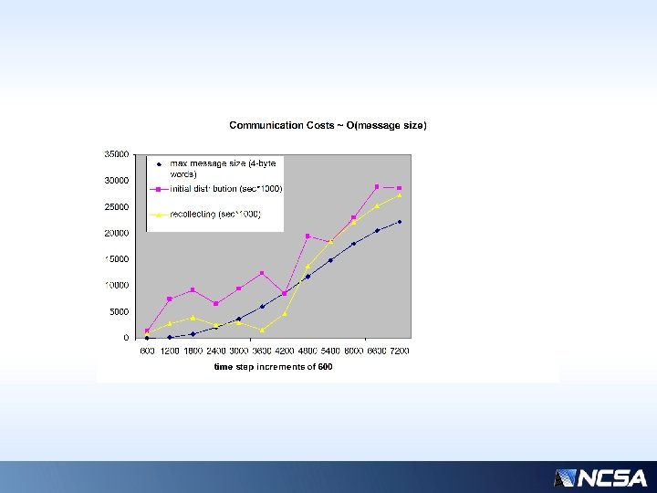
Communication Costs as a Function of Message Sizes • Number of receivers actually decreases later in this small simulation because more processors are developing their own work – so actually fewer distribution (and hence recollecting) messages as the overall workload increases. (This effect would be MUCH smaller on larger processor counts. ) • Comm costs do not correlate well with message sizes early on; then becomes limited at ~4200 steps • This test case is 32 processors, nx=ny=96 nz=596 dx=dy=1000 dz=100 Local size is 24 x 12 (nprocx=4, nprocy=8)

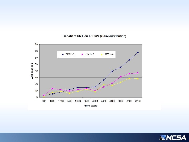
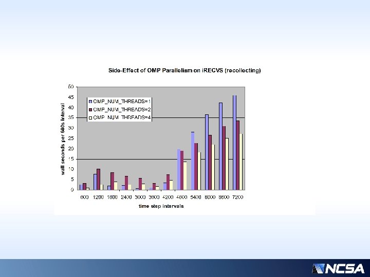
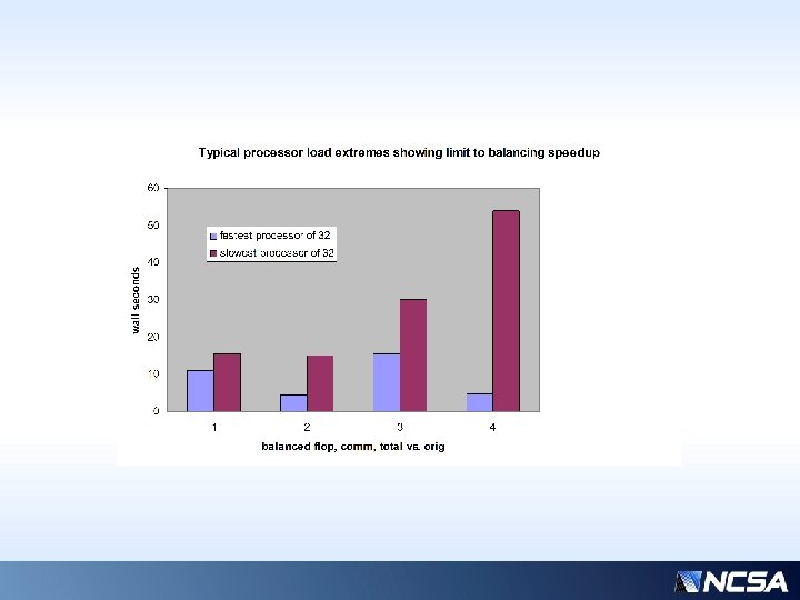
Positive Side-effect of SMT on Messaging • Notice that communication-wait performance also responds dramatically to SMT concurrency, even though the messaging itself is not contained in a parallel region. • Shows sensitivity of communication wait latencies on “flops” workload per processor

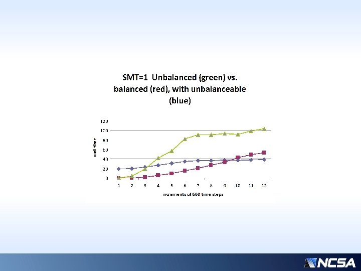
Previous slide… • Over a typical time interval (4200 -4800 s), the component times of the slowest/fastest processors are shown. • “common” times (those that are not balanceable, constant, or insignificant) have been removed for clarity • Assuming performance is limited by the slowest processor, even with nearly ideal balancing, we could only hope for ~3 x speedup… (~50 / ~15 ) * • But there is comm overhead (column 2)… • Actual realizable speedup is more like 5/3 • * Why only 3 x? For only 32 processors, this is highly sensitive to the average workload distribution…

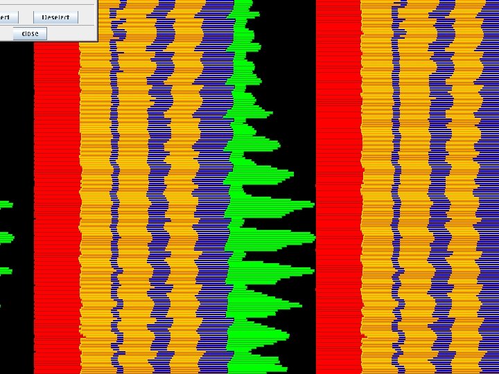
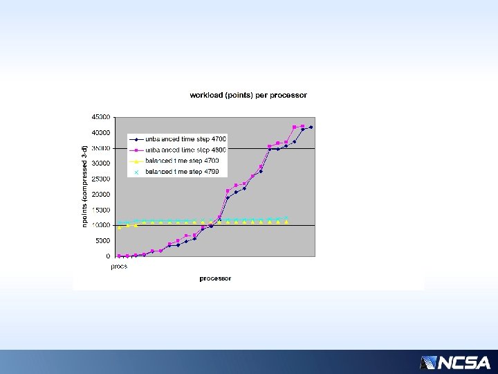
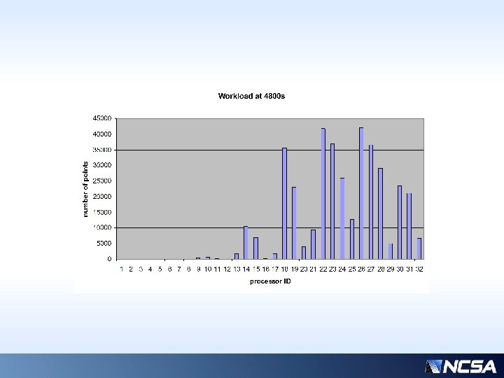
Next Slide: Snapshot of workload distribution • 32 processors • Snapshot at 4800 s • For timing examples, processor ID=21 shows to be the most expensive, and 14, the least, so we’ll focus on just those two, at a representative time step. • #21 is a “sender” (to procs 0, 6, 28) and #14 is a “receiver” (from proc 25) • All other processors’ time stamps fall on curves bracketed by 14 and 21

Time stamps for phases of MP (unbalanced version) showing fastest (blue) vs. slowest (red) processors

Various phases used in timing diagrams 1 end init 15 end of waits 1 16 end of flops 2 2 end of calcl 1 17 end of waits 2 3 end of calc 2 18 end of flops 3 4 end of preload 1 19 end of waits 3 5 Not used 6 Not used 20 N. A. 21 end of flops 4 7 end of preload 2 22 end of isend back 8 end of global 23 end of flops 5 9 end of heur 24 end of mpi_test 25 end of final recv back wait 26 end of send back waits 27 end of rescatter arrays 10 end of isends 1 11 end of start of irecv back 12 13 14 end of probes end of blocking first recvs end of flops 1

Gaps between colors indicate time disparity for processors at a certain phase; note serious lag in final receive phase, minor lag at early receive phase. Perfectly overlaid lines indicates they are running in lock-step.

Interpretation of previous slides… • Goal is that all procs start with nearly identical time stamps, and finish at some later identical time stamp • This would show that nobody is wasting time waiting for lack of work, or on communication • Ideally, all intermediate phase time stamps would also be coincident • Need to minimize the necessary initial delay between senders and receivers, and hide as much as possible the delay for the reverse communication on the back end • Goal: Narrow the envelope between the MIN, MAX processors. The better these two curves can be aligned, with all others procs in between, the better the balance.

So why is the receive-back so expensive? • Note that the non-blocking receives for the final regathering of “borrowed” work are posted very early on; right after the initial isends, in fact. • The plan was to have the latency for these receives hidden by the pure compute work… BUT notice that the absolute value of the pure work “flops” is a relatively flat line, indicating not much time is spent there anyway • Let’s try an experiment: add some bogus work to simulate a more intense MP kernel. E. g. : • work = nstep*work*dot_product (qhw(1: ngscnt), qsw(1: ngscnt)) • (repeat as needed… 4 times was optimal in this case)

Effect of adding extra work ONLY to procs 14 and 21

All processors given extra work BEFORE i. SENDs… #14 is now the max time

Effect of adding extra work to ALL procs AFTER i. SENDs; #14 is now delayed for having to wait on sends to #25.

Previous slides… • Major delay in sender (at phase 19) is due to waiting on the send-back to be received by proc #25 • Major delay in both procs (at phase 23) is the extra flops work, as expected • Why should proc 14 have this new delay? His actual communication partner is #25, (not #21), so adding extra work universally has side effects… • I believe this makes a case that communication costs can be successfully mitigated by an informed distribution of work (not necessarily equal work) because the communication burden is not equally shared

So what should we reasonably expect for latency and/or B/W delays? • Next slide – test of OSU benchmark suite… • Where do we fall on these curves ?

Results of OSU latency and bandwidth tests: Even the worst case (4 MB) only has latency of 0. 002 s ; LFO messages typically ~10, 000 4 -byte reals (x 12 for full send back). Does not explain the latency delays observed, which are O(10 x) greater.

Nice paper from Sandia on MPI overhead and overlap in applications: • • • Measuring MPI Send and Receive Overhead and Application Availability in High Performance Network Interfaces (http: //citeseerx. ist. psu. edu/viewdoc/download? doi=10. 1. 1. 112. 537&rep=rep 1&type=pdf) Douglas Doerfler and Ron Brightwell. Center for Computation, Computers, Information and Math. Sandia National Laboratories 1. Albuquerque, NM 87185 -0817. . . This paper discusses the critical threshold values for message sizes and overlapped work to determine the actual MPI overhead for message transfers, and introduces application availability as the fraction of total transfer time that the application is free to perform non -MPI related work Protocol boundary significance (i. e. ~32 K bytes) Overlap potentially beneficial for codes that send multiple small messages; not so much so if transfer time is relatively small, with small message size

Conclusions • Not a solved problem… speedups disappointing so far. • • “Serial” computation overhead Communication overhead • Processor core speed versus network latency/bandwidth will produce a wide variety of balancing profiles • May need more complicated tricks like using points from previous time step if latency cannot be hidden by legitimate work • It is not as simple as aiming to have each processor work on the same number of points because the (unequal) costs of transferring that data must be considered • At “scale”, all of these effects expect to be magnified • Demonstrated sensitivity to work quanta between communications

Extensibility of the model • Most easily extended to Morrison since code is already written with large IF blocks for micro • WSM 5, 6 are more complicated because IF conditions need to be pulled out of many small blocks with irregular structure and arrays would need to be gathered/compressed • Want to be confident in proof of concept with LFOICE first

Current and future work • Carry out these same profiling and timing techniques “at scale” on larger systems • Fewer “senders” with many more “receiver” partners • Topology-aware distribution? • Communication costs to vary even more across distant procs… • Improve feedback to include communication times such as those shown by the stamps here • Want to test if more computationally intensive MP kernels might show more potential for speedup from balancing

Questions? • Please email me for follow-up, source code, testing, etc. : ms@ncsa. illinois. edu