Advanced applications of artificial neural networks In 1990

Advanced applications of artificial neural networks In 1990 s, ANNs are de-mystified • ANN joins ranks of non-parametric statistical methods • Back propagation is recognized as non-biological In 2000 s • Genome sequencing stimulates increase in data-mining • New methods of data mining start replacing ANN In 2010 s Neural Networks make a comeback in the Big-Data era with Deep Learning • Beware of treating ANN as a black box • Review some unusual aspects of ANN

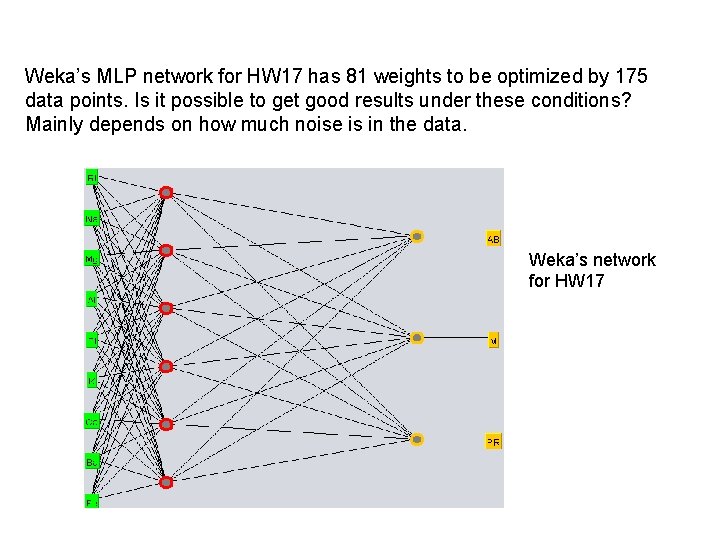
Weka’s MLP network for HW 17 has 81 weights to be optimized by 175 data points. Is it possible to get good results under these conditions? Mainly depends on how much noise is in the data. Weka’s network for HW 17

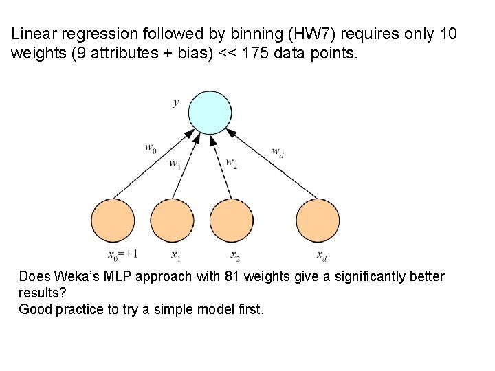
Linear regression followed by binning (HW 7) requires only 10 weights (9 attributes + bias) << 175 data points. Does Weka’s MLP approach with 81 weights give a significantly better results? Good practice to try a simple model first.

Application of validation sets to MLPs reduces the data available for weight optimization. In polynomial regression the validation subset can be returned to training set after the best degree has been determined. With MLPs, we cannot expect the results revealed by a validation set to hold if back propagation is repeated with new training set that is old training set + validation set. With MLP back propagation, Eval is more like Etest, examples never used in training.

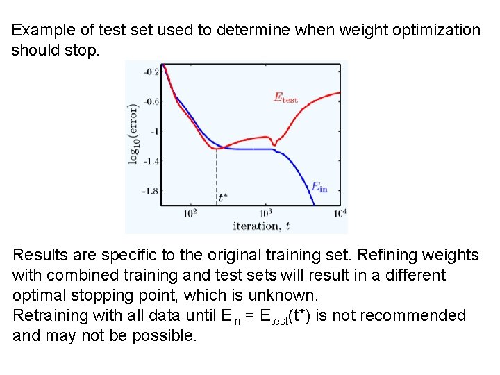
Example of test set used to determine when weight optimization should stop. Results are specific to the original training set. Refining weights with combined training and test sets will result in a different optimal stopping point, which is unknown. Retraining with all data until Ein = Etest(t*) is not recommended and may not be possible.

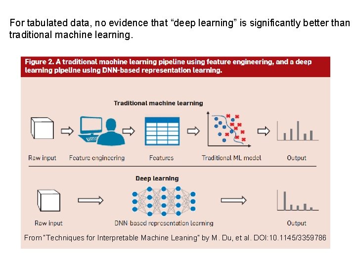
For tabulated data, no evidence that “deep learning” is significantly better than traditional machine learning. From “Techniques for Interpretable Machine Leaning” by M. Du, et al. DOI: 10. 1145/3359786

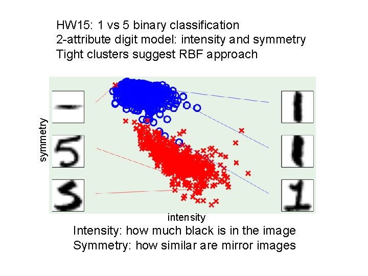
symmetry HW 15: 1 vs 5 binary classification 2 -attribute digit model: intensity and symmetry Tight clusters suggest RBF approach intensity Intensity: how much black is in the image Symmetry: how similar are mirror images

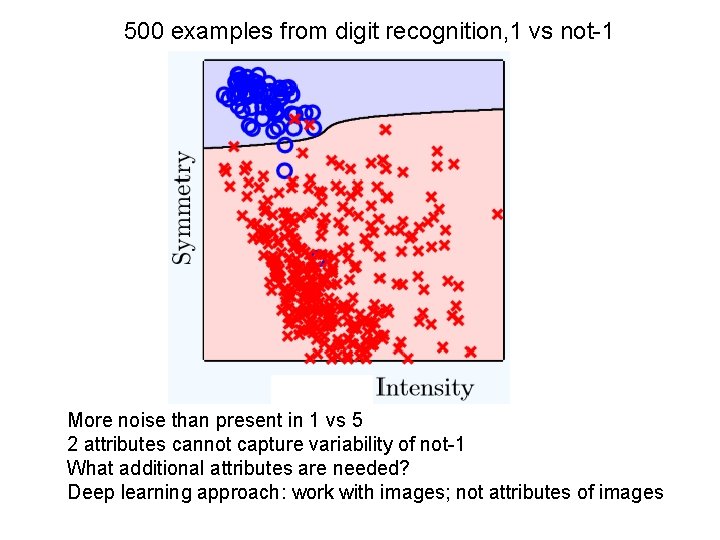
500 examples from digit recognition, 1 vs not-1 More noise than present in 1 vs 5 2 attributes cannot capture variability of not-1 What additional attributes are needed? Deep learning approach: work with images; not attributes of images

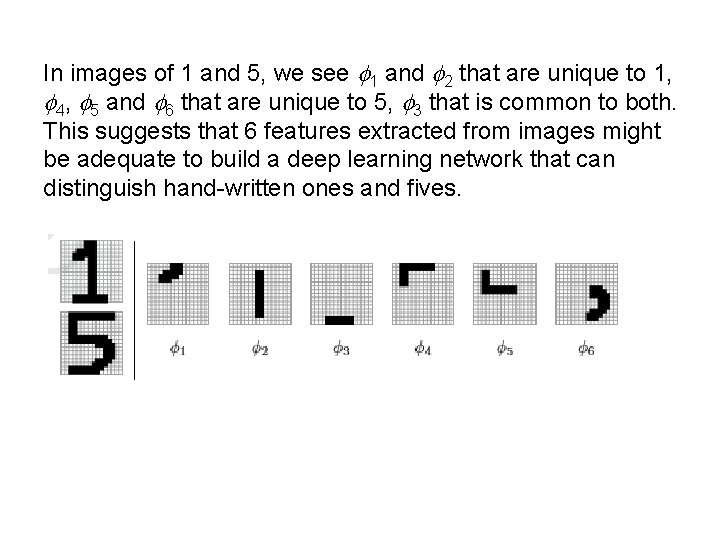
In images of 1 and 5, we see f 1 and f 2 that are unique to 1, f 4, f 5 and f 6 that are unique to 5, f 3 that is common to both. This suggests that 6 features extracted from images might be adequate to build a deep learning network that can distinguish hand-written ones and fives.

Rationale of a “deep learning” network to distinguish 1 from 5 Input 16 x 16 pixel images. First hidden layer extracts features from data. Second hidden layer merges features. z 1 increases if f 1 and f 2 are present and f 4 through f 6 are absent. z 5 increases if f 1 and f 2 are absent and f 4 through f 6 are present. Output is binary classification of z 1 and z 5

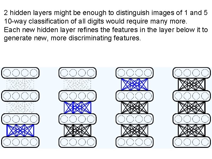
2 hidden layers might be enough to distinguish images of 1 and 5 10 -way classification of all digits would require many more. Each new hidden layer refines the features in the layer below it to generate new, more discriminating features.

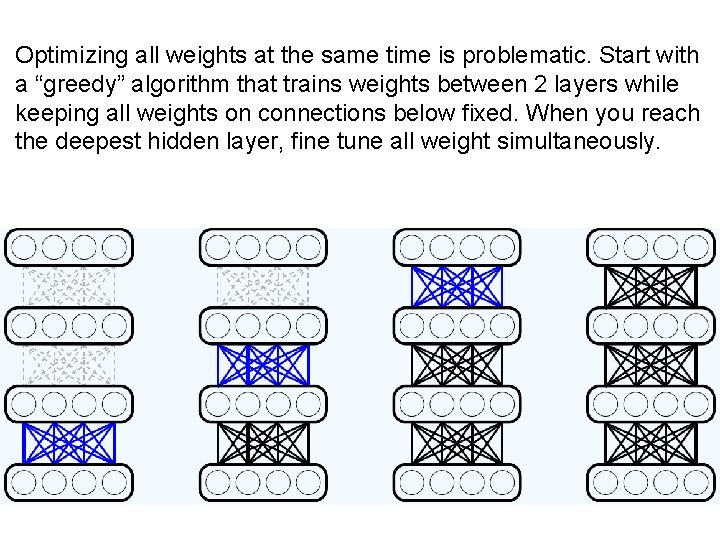
Optimizing all weights at the same time is problematic. Start with a “greedy” algorithm that trains weights between 2 layers while keeping all weights on connections below fixed. When you reach the deepest hidden layer, fine tune all weight simultaneously.

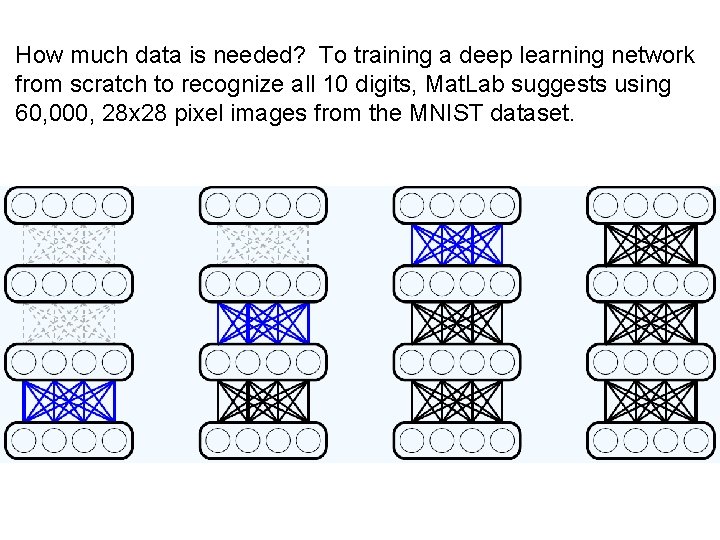
How much data is needed? To training a deep learning network from scratch to recognize all 10 digits, Mat. Lab suggests using 60, 000, 28 x 28 pixel images from the MNIST dataset.

Convolutional Neural Networks (CNNs): highly developed deep leaning networks for image processing

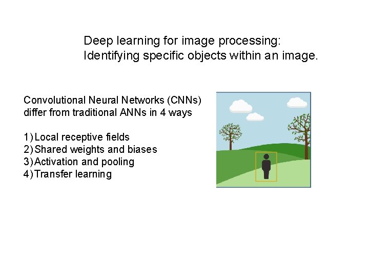
Deep learning for image processing: Identifying specific objects within an image. Convolutional Neural Networks (CNNs) differ from traditional ANNs in 4 ways 1) Local receptive fields 2) Shared weights and biases 3) Activation and pooling 4) Transfer learning

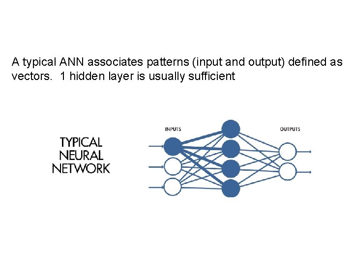
A typical ANN associates patterns (input and output) defined as vectors. 1 hidden layer is usually sufficient

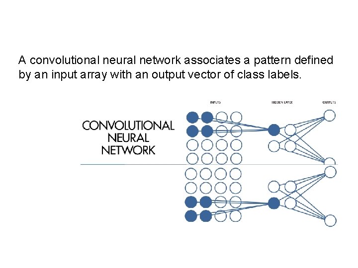
A convolutional neural network associates a pattern defined by an input array with an output vector of class labels.

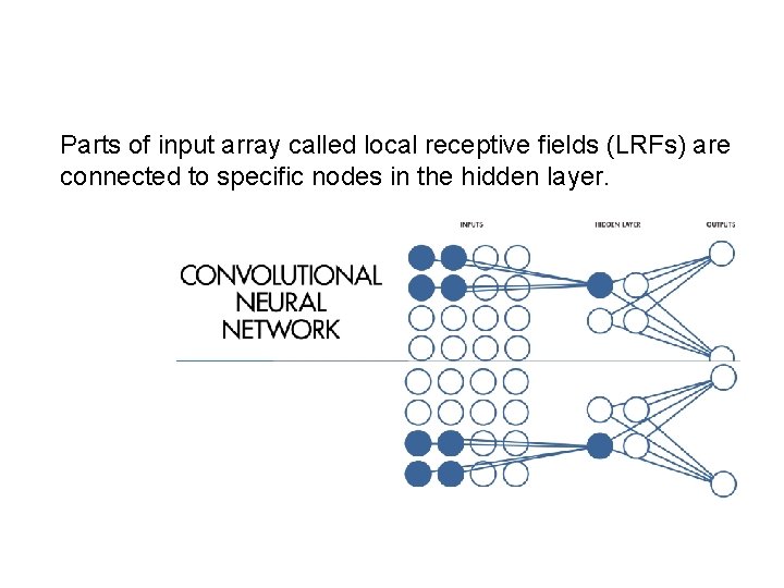
Parts of input array called local receptive fields (LRFs) are connected to specific nodes in the hidden layer.

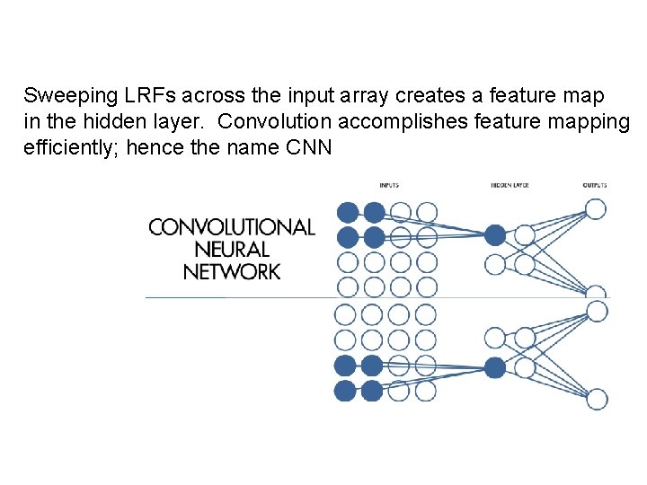
Sweeping LRFs across the input array creates a feature map in the hidden layer. Convolution accomplishes feature mapping efficiently; hence the name CNN

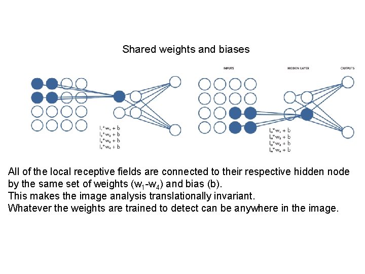
Shared weights and biases All of the local receptive fields are connected to their respective hidden node by the same set of weights (w 1 -w 4) and bias (b). This makes the image analysis translationally invariant. Whatever the weights are trained to detect can be anywhere in the image.

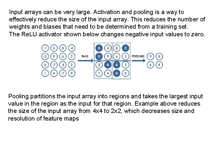
Input arrays can be very large. Activation and pooling is a way to effectively reduce the size of the input array. This reduces the number of weights and biases that need to be determined from a training set. The Re. LU activator shown below changes negative input values to zero. Pooling partitions the input array into regions and takes the largest input value in the region as the input for that region. Example above reduces the size of the input array from 4 x 4 to 2 x 2, which decreases size and resolution of feature maps

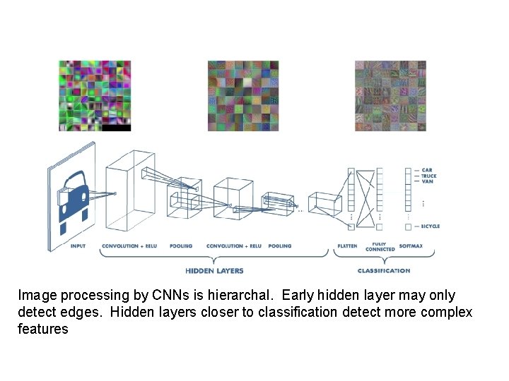
CNNs have many hidden layer to obtain feature maps of many input regions After many cycles of convolution, Re. LU activation, and pooling for multiple regions of the image, feature maps are classified to obtain class likelihoods. In example shown below, likelihood of car should be mush greater than likelihood of other classes.

Image processing by CNNs is hierarchal. Early hidden layer may only detect edges. Hidden layers closer to classification detect more complex features

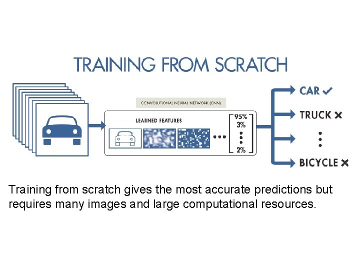
Training from scratch gives the most accurate predictions but requires many images and large computational resources.

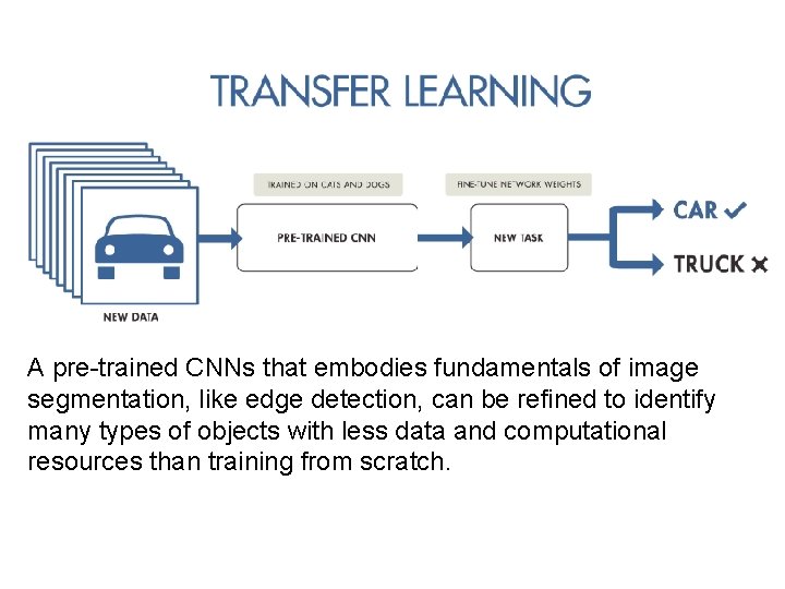
A pre-trained CNNs that embodies fundamentals of image segmentation, like edge detection, can be refined to identify many types of objects with less data and computational resources than training from scratch.

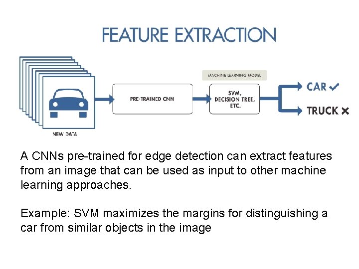
A CNNs pre-trained for edge detection can extract features from an image that can be used as input to other machine learning approaches. Example: SVM maximizes the margins for distinguishing a car from similar objects in the image