Advanced Algorithms Piyush Kumar Lecture 16 Parallel Algorithms
 Welcome to COT 5405 Courtesy Baker")


")


=1 Rank(3)=1 Rank(10)=2 Rank(15)=4 Rank(16)=4")
 = T(n/2) + O(log n) • Using the idea")

 { Compute separation line L such")
 { Compute separation line L such")
 • HL = Merge. Hull( Left")


) 1. 2. 3. – – – 4. Sort the")


 , and polygons to the")
 time. • Step 2: Partition")
 = t( n)")
- Slides: 34
Advanced Algorithms Piyush Kumar (Lecture 16: Parallel Algorithms) Welcome to COT 5405 Courtesy Baker 05.
Parallel Models • An abstract description of a real world parallel machine. • Attempts to capture essential features (and suppress details? ) • What other models have we seen so far? RAM? External Memory Model?
RAM • Random Access Machine Model – Memory is a sequence of bits/words. – Each memory access takes O(1) time. – Basic operations take O(1) time: Add/Mul/Xor/Sub/AND/not… – Instructions can not be modified. – No consideration of memory hierarchies. – Has been very successful in modelling real world machines.
Parallel RAM aka PRAM • Generalization of RAM • P processors with their own programs (and unique id) • MIMD processors : At each point in time the processors might be executing different instructions on different data. • Shared Memory • Instructions are synchronized among the processors
PRAM Shared Memory EREW/ERCW/CREW/CRCW EREW: A program isnt allowed to access the same memory location at the same time.
Variants of CRCW • Common CRCW: CW iff processors write same value. • Arbitrary CRCW • Priority CRCW • Combining CRCW
Why PRAM? • Lot of literature available on algorithms for PRAM. • One of the most “clean” models. • Focuses on what communication is needed ( and ignores the cost/means to do it) • Most ideas translate to other models.
Problems with PRAM • Unrealistic – Constant time memory access? • Fixed number of processors
PRAM Algorithm design. • Problem 1: Produce the sum of an array of n numbers. • RAM = ? • PRAM = ?
Problem 2: Prefix Computation Let X = {s 0, s 1, …, sn-1} be in a set S Let Ä be a binary, associative, closed operator with respect to S (usually Q(1) time – MIN, MAX, AND, +, . . . ) The result of s 0Ä s 1 Ä…Ä sk is called the k-th prefix Computing all such n prefixes is the parallel prefix computation 1 st prefix 2 nd prefix 3 rd prefix. . . (n-1)th prefix s 0 Ä s 1 Ä s 2. . . s 0 Ä s 1 Ä. . . Ä sn-1
Prefix computation • Suffix computation is a similar problem. • Assumes Binary op takes O(1) • In RAM = ?
Prefix Computation (Akl)
EREW PRAM Prefix computation • Assume PRAM has n processors and n is a power of 2. • Input: si for i = 0, 1, . . . , n-1. • Algorithm Steps: for j = 0 to (lg n) -1, do for i = 2 j to n-1 do h = i - 2 j si = s h Ä si endfor Total time in EREW PRAM?
Problem 3: Array packing • Assume that we have – an array of n elements, X = {x 1, x 2, . . . , xn} – Some array elements are marked (or distinguished). • The requirements of this problem are to – pack the marked elements in the front part of the array. – place the remaining elements in the back of the array. • While not a requirement, it is also desirable to – maintain the original order between the marked elements – maintain the original order between the unmarked elements
In RAM? • • How would you do this? Inplace? Running time? Any ideas on how to do this in PRAM?
EREW PRAM Algorithm 1. Set si in Pi to 1 if xi is marked and set si = 0 otherwise. 2. Perform a prefix sum on S =(s 1, s 2 , . . . , sn) to obtain destination di = si for each marked xi. 3. All PEs set m = sn , the total nr of marked elements. 4. Pi sets si to 0 if xi is marked and otherwise sets si = 1. 5. Perform a prefix sum on S and set di = si + m for each unmarked xi. 6. Each Pi copies array element xi into address di in X.
Array Packing • Assume n processors are used above. • Optimal prefix sums requires O(lg n) time. • The EREW broadcast of sn needed in Step 3 takes O(lg n) time using a binary tree in memory • All and other steps require constant time. • Runs in O(lg n) time and is cost optimal. • Maintains original order in unmarked group as well Notes: • Algorithm illustrates usefulness of Prefix Sums • There many applications for Array Packing algorithm
Problem 4: PRAM Merge. Sort • RAM Merge Sort Recursion? • PRAM Merge Sort recursion? • Can we speed up the merging? – Merging n elements with n processors can be done in O(log n) time. – Assume all elements are distinct – Rank(a, A) = number of elements in A smaller than a. For example rank(8, {1, 3, 5, 7, 9}) = 4
PRAM Merging A = 2, 3, 10, 15, 16 Rank(2)=1 Rank(3)=1 Rank(10)=2 Rank(15)=4 Rank(16)=4 1 2 3 B = 1, 8, 12, 14, 19 +1 +2 +3 +4 +5 8 10 Rank(1)=0 Rank(8)=2 Rank(12)=3 Rank(14)=3 Rank(19)=5 12 14 15 16 19 +1 +2 +3 +4 +5
PRAM Merge Sort • T(n) = T(n/2) + O(log n) • Using the idea of pipelined d&c PRAM Mergesort can be done in O(log n). • D&C is one of the most powerful techniques to solve problems in parallel.
Problem 5: Closest Pair • RAM Version ? L 7 6 4 12 5 = min(12, 21) 3 2 1 21
Closest Pair: RAM Version Closest-Pair(p 1, …, pn) { Compute separation line L such that half the points are on one side and half on the other side. 1 = Closest-Pair(left half) 2 = Closest-Pair(right half) = min( 1, 2) 2 T(n / 2) Delete all points further than from separation line L O(n) Sort remaining points by y-coordinate. O(n log n) Scan points in y-order and compare distance between each point and next 11 neighbors. If any of these distances is less than , update . O(n) return . } O(n log n)
Closest Pair: PRAM Version? Closest-Pair(p 1, …, pn) { Compute separation line L such that half the points are on one side and half on the other side. Use sorted lists 1 = Closest-Pair(left half) 2 = Closest-Pair(right half) = min( 1, 2) In parallel O(1) T(n / 2) Delete all points further than from separation line L Sort remaining points by y-coordinate. Use presorting and prefix computation. Scan points in y-order and compare distance between each point and next 11 neighbors. Find min of all these distances, update . return . } Again use prefix computation. O(log n) O(1) O(log n) Recurrence : T(n) = T(n/2) + O(log n)
Problem 6: Planar Convex hulls Merge. Hull (P) • HL = Merge. Hull( Left of median) • HR = Merge. Hull( Right of median) • Return Join. Hulls(HL, HR) Time complexity in RAM? Time complexity in PRAM?
Join_Hulls
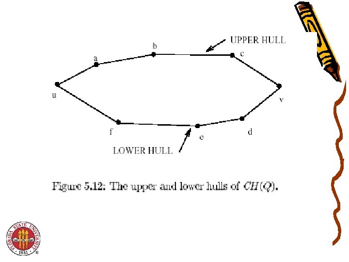
Towards a better Planar Convex hull • Let Q = {q 1, q 2, . . . , qn} be a set of points in the Euclidean plane (i. e. , E 2 -space). • The convex hull of Q is denoted by CH(Q) and is the smallest convex polygon containing Q. • – It is specified by listing its corner points (which are from Q) in order (e. g. , clockwise order). Usual Computational Geometry Assumptions: – – – No three points lie on the same straight line. No two points have the same x or y coordinate. There at least 4 points, as CH(Q) = Q for n 3.
PRAM CONVEX HULL(n, Q, CH(Q)) 1. 2. 3. – – – 4. Sort the points of Q by x-coordinate. Partition Q into k = n subsets Q 1, Q 2, . . . , Qk of k points each such that a vertical line can separate Qi from Qj Also, if i < j, then Qi is left of Qj. For i = 1 to k , compute the convex hulls of Qi in parallel, as follows: if |Qi| 3, then CH(Qi) = Qi else (using k= n PEs) call PRAM CONVEX HULL(k, Qi, CH(Qi)) Merge the convex hulls in {CH(Q 1), CH(Q 2), . . . , CH(Qk)} together.
Basic Idea
Last Step • The upper hull is found first. Then, the lower hull is found next using the same method. – Only finding the upper hull is described here – Upper & lower convex hull points merged into ordered set • Each CH(Qi) has n PEs assigned to it. • The PEs assigned to CH(Qi) (in parallel) compute the upper tangent from CH(Qi) to another CH(Qj). – A total of n-1 tangents are computed for each CH(Qi) – Details for computing the upper tangents will be separately
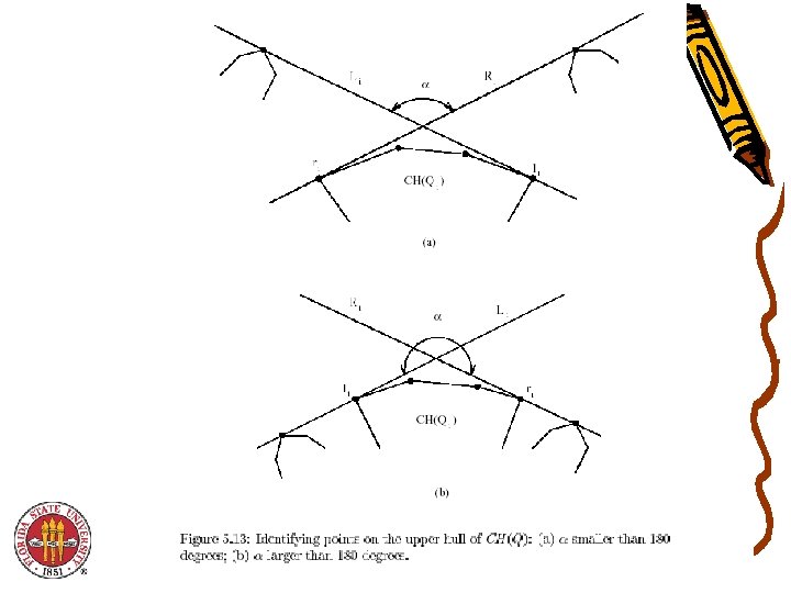
Last Step • Among the tangent lines to CH(Qi) , and polygons to the left of CH(Qi), let Li be the one with the smallest slope. • Among the tangent lines to CH(Qi) and polygons to the right, let Ri be the one with the largest slope. • If the angle between Li and Ri is less than 180 degrees, no point of CH(Qi) is in CH(Q). • – See Figure 5. 13 on next slide (from Akl’s Online text) – Otherwise, all points in CH(Q) between where Li touches CH(Qi) and where Ri touches CH(Qi) are in CH(Q). Array Packing is used to combine all convex hull points of CH(Q) after they are identified.
Complexity • Step 1: The sort takes O(lg n) time. • Step 2: Partition of Q into subsets takes O(1) time. • Step 3: The recursive calculations of CH(Qi) for 1 i n in parallel takes t(n) time (using n PEs for each Qi). • Step 4: The big steps here require O(lgn) and are – Finding the upper tangent from CH(Qi) to CH(Qj) for each i, j pair. – Array packing used to form the ordered sequence of upper convex hull points for Q. • Above steps find the upper convex hull. The lower convex hull is found similarly. – Upper & lower hulls merged in O(1) time to ordered set
Complexity • Cost for Step 3: Solving the recurrance relation t(n) = t( n) + lg n yields t(n) = O(lg n) • Running time for PRAM Convex Hull is O(lg n) since this is maximum cost for each step. • Then the cost for PRAM Convex Hull is C(n) = O(n lg n).