Advanced Algorithms Piyush Kumar Lecture 11 Div Conquer

Advanced Algorithms Piyush Kumar (Lecture 11: Div & Conquer) Welcome to COT 5405 Source: Kevin Wayne, Harold Prokop.

Divide and Conquer • • • Inversions Closest Point problems Integer multiplication Matrix Multiplication Cache Aware algorithms/ Cache oblivious Algorithms • Static Van Emde Boas Layout

5. 3 Counting Inversions

Counting Inversions • Music site tries to match your song preferences with others. – You rank n songs. – Music site consults database to find people with similar tastes. • Similarity metric: number of inversions between two rankings. – My rank: 1, 2, …, n. – Your rank: a 1, a 2, …, an. – Songs i and j inverted if i < j, but ai > aj. Songs • A B C D E Inversions Me 1 2 3 4 5 3 -2, 4 -2 You 1 3 4 2 5 Brute force: check all (n 2) pairs i and j.

• Applications. – – – Voting theory. Collaborative filtering. Measuring the "sortedness" of an array. Sensitivity analysis of Google's ranking function. Rank aggregation for meta-searching on the Web. Nonparametric statistics (e. g. , Kendall's Tau distance).

Counting Inversions: Divide-and-Conquer • Divide-and-conquer. 1 5 4 8 10 2 6 9 12 11 3 7

Counting Inversions: Divide-and-Conquer • Divide-and-conquer. – Divide: separate list into two pieces. 1 1 5 5 4 4 8 8 10 10 2 2 6 6 9 9 12 12 11 11 3 3 7 7 Divide: O(1).

Counting Inversions: Divide-and-Conquer • Divide-and-conquer. 1 1 – Divide: separate list into two pieces. – Conquer: recursively count inversions in Divide: O(1). 5 4 8 10 2 6 9 12 11 3 7 each half. 5 4 8 10 5 blue-blue inversions 5 -4, 5 -2, 4 -2, 8 -2, 10 -2 2 6 9 12 11 3 7 Conquer: 2 T(n / 2) 8 green-green inversions 6 -3, 9 -7, 12 -3, 12 -7, 12 -11, 11 -3, 11 -7

Counting Inversions: Divide-and-Conquer • Divide-and-conquer. – Divide: separate list into two pieces. – Conquer: recursively count inversions in each half. – Combine: count inversions where ai and aj are in different halves, and return sum of three quantities. 1 1 5 5 4 4 8 8 10 10 2 2 6 6 5 blue-blue inversions 9 9 12 12 11 3 3 7 7 Divide: O(1). Conquer: 2 T(n / 2) 8 green-green inversions 9 blue-green inversions 5 -3, 4 -3, 8 -6, 8 -3, 8 -7, 10 -6, 10 -9, 10 -3, 10 -7 Total = 5 + 8 + 9 = 22. 11 Combine: ? ? ?

Counting Inversions: Combine • Combine: count blue-green inversions – Assume each half is sorted. to maintain sorted invariant – Count inversions where ai and aj are in different halves. – Merge two sorted halves into sorted whole. • 3 7 10 14 18 19 2 11 16 17 23 25 6 3 2 2 0 0 13 blue-green inversions: 6 + 3 + 2 + 0 2 3 7 10 11 14 16 17 18 19 Count: O(n) 23 25 Merge: O(n)

Counting Inversions: Implementation • • Pre-condition. [Merge-and-Count] A and B are sorted. Post-condition. [Sort-and-Count] L is sorted. Sort-and-Count(L) { if list L has one element return 0 and the list L Divide the list into two halves A and B (r. A, A) Sort-and-Count(A) (r. B, B) Sort-and-Count(B) (r. B, L) Merge-and-Count(A, B) } return r = r. A + r. B + r and the sorted list L

5. 4 Closest Pair of Points 12

Closest Pair of Points • Closest pair. Given n points in the plane, find a pair with smallest Euclidean distance between them. • Fundamental geometric primitive. – Graphics, computer vision, geographic information systems, molecular modeling, air traffic control. – Special case of nearest neighbor, Euclidean MST, Voronoi. fast closest pair inspired fast algorithms for these problems • Brute force. Check all pairs of points p and q with (n 2) comparisons. • 1 -D version. O(n log n) easy if points are on a line. • Assumption. No two points have same x coordinate. to make presentation cleaner

Closest Pair of Points: First Attempt • Divide. Sub-divide region into 4 quadrants. L

Closest Pair of Points: First Attempt • • Divide. Sub-divide region into 4 quadrants. Obstacle. Impossible to ensure n/4 points in each piece. L

Closest Pair of Points • Algorithm. – Divide: draw vertical line L so that roughly ½n points on each side. L

Closest Pair of Points • Algorithm. – Divide: draw vertical line L so that roughly ½n points on each side. – Conquer: find closest pair in each side recursively. L 21 12

Closest Pair of Points • Algorithm. – Divide: draw vertical line L so that roughly ½n points on each side. – Conquer: find closest pair in each side recursively. – Combine: find closest pair with one point in each side. – Return best of 3 solutions. L 8 12 21 seems like (n 2)

Closest Pair of Points • Find closest pair with one point in each side, assuming that distance < . L 21 12 = min(12, 21)

Closest Pair of Points • Find closest pair with one point in each side, assuming that distance < . – Observation: only need to consider points within of line L. L 21 = min(12, 21) 12

Closest Pair of Points • Find closest pair with one point in each side, assuming that distance < . – Observation: only need to consider points within of line L. – Sort points in 2 -strip by their y coordinate. L 7 6 4 12 5 21 = min(12, 21) 3 2 1

Closest Pair of Points • Find closest pair with one point in each side, assuming that distance < . – Observation: only need to consider points within of line L. – Sort points in 2 -strip by their y coordinate. – Only check distances of those within 11 positions in sorted list! L 7 6 4 12 5 21 = min(12, 21) 3 2 1

Closest Pair of Points • • • Def. Let si be the point in the 2 -strip, with the ith smallest y-coordinate. Claim. If |i – j| 12, then the distance between si and sj is at least . Pf. – No two points lie in same ½ -by-½ box. 2 rows – Two points at least 2 rows apart have distance 2(½ ). ▪ i • j 39 31 ½ ½ 30 29 28 27 Fact. Still true if we replace 12 with 7. 26 25 ½

Closest Pair Algorithm Closest-Pair(p 1, …, pn) { Compute separation line L such that half the points are on one side and half on the other side. 1 = Closest-Pair(left half) 2 = Closest-Pair(right half) = min( 1, 2) 2 T(n / 2) Delete all points further than from separation line L O(n) Sort remaining points by y-coordinate. O(n log n) Scan points in y-order and compare distance between each point and next 11 neighbors. If any of these distances is less than , update . O(n) return . } O(n log n)

Closest Pair of Points: Analysis • Running time. • Q. Can we achieve O(n log n)? • A. Yes. Don't sort points in strip from scratch each time. – Each recursive returns two lists: all points sorted by y coordinate, and all points sorted by x coordinate. – Sort by merging two pre-sorted lists.

5. 5 Integer Multiplication 26

Integer Arithmetic • Add. Given two n-digit integers a and b, compute a + b. – O(n) bit operations. • Multiply. Given two n-digit integers a and b, compute a × b. – Brute force solution: (n 2) bit operations. 1 1 0 1 0 1 * 0 1 1 1 0 1 0 Multiply 0 0 0 0 0 1 1 0 1 0 1 1 1 0 1 0 1 + 0 1 1 1 0 1 0 1 0 Add 1 1 0 1 0 1 1 0 1 0 0 0 0 0 0 1 0

Divide-and-Conquer Multiplication: Warmup • To multiply two n-digit integers: – Multiply four ½n-digit integers. – Add two ½n-digit integers, and shift to obtain result. assumes n is a power of 2

Karatsuba Multiplication • To multiply two n-digit integers: – Add two ½n digit integers. – Multiply three ½n-digit integers. – Add, subtract, and shift ½n-digit integers to obtain result. A • B A C C Theorem. [Karatsuba-Ofman, 1962] Can multiply two n-digit integers in O(n 1. 585) bit operations.

Karatsuba: Recursion Tree n T(n) T(n/2) 3(n/2) T(n/4) T(n/4) T(n/4) 9(n/4) . . . 3 k (n / 2 k) T(n / 2 k) . . . T(2) T(2) 3 lg n (2)

Matrix Multiplication 31

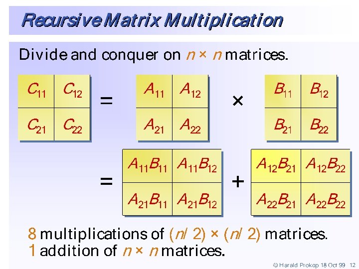
Courtesy Harold Prokop Matrix Multiplication (MM) n cij = ∑ a ik bkj k =1 × = C A B

Matrix Multiplication • Matrix multiplication. Given two n-by-n matrices A and B, compute C = AB. • Brute force. (n 3) arithmetic operations. • Fundamental question. Can we improve upon brute force?

Matrix Multiplication: Warmup • Divide-and-conquer. – Divide: partition A and B into ½n-by-½n blocks. – Conquer: multiply 8 ½n-by-½n recursively. – Combine: add appropriate products using 4 matrix additions.

Matrix Multiplication: Key Idea • Key idea. multiply 2 -by-2 block matrices with only 7 multiplications. – 7 multiplications. – 18 = 10 + 8 additions (or subtractions).

Fast Matrix Multiplication • Fast matrix multiplication. (Strassen, 1969) – Divide: partition A and B into ½n-by-½n blocks. – Compute: 14 ½n-by-½n matrices via 10 matrix additions. – Conquer: multiply 7 ½n-by-½n matrices recursively. – Combine: 7 products into 4 terms using 8 matrix additions. • Analysis. – Assume n is a power of 2. – T(n) = # arithmetic operations.

Fast Matrix Multiplication in Practice • Implementation issues. – Sparsity. – Caching effects. – Numerical stability. – Odd matrix dimensions. – Crossover to classical algorithm around n = 128. • Common misperception: "Strassen is only a theoretical curiosity. " – Advanced Computation Group at Apple Computer reports 8 x speedup on G 4 Velocity Engine when n ~ 2, 500. – Range of instances where it's useful is a subject of controversy. • Remark. Can "Strassenize" Ax=b, determinant, eigenvalues, and other matrix ops.

Fast Matrix Multiplication in Theory • • Q. Multiply two 2 -by-2 matrices with only 7 scalar multiplications? A. Yes! [Strassen, 1969] • • Q. Multiply two 2 -by-2 matrices with only 6 scalar multiplications? A. Impossible. [Hopcroft and Kerr, 1971] • • Q. Two 3 -by-3 matrices with only 21 scalar multiplications? A. Also impossible. • • Q. Two 70 -by-70 matrices with only 143, 640 scalar multiplications? A. Yes! [Pan, 1980] • Decimal wars. – December, 1979: O(n 2. 521813). – January, 1980: O(n 2. 521801).

Fast Matrix Multiplication in Theory • Best known. O(n 2. 376) [Coppersmith. Winograd, 1987. ] • Conjecture. O(n 2+ ) for any > 0. • Caveat. Theoretical improvements to Strassen are progressively less practical.

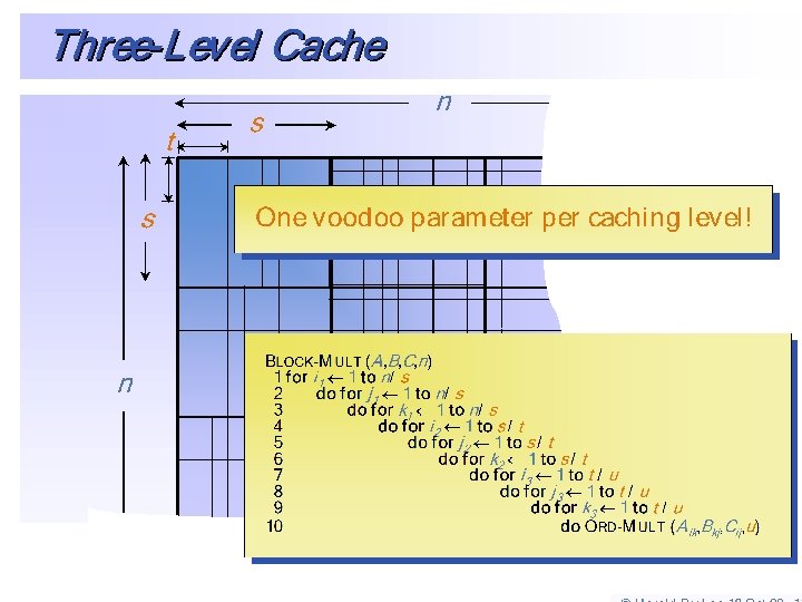
Cache - Aware MM BBLOCK-M ULT(A -MULT (A, B, C, n) 11 for ¬ 11 to for ii¬ to n/ n/ ss 22 do ¬ 11 to do for jj¬ to n/ n/ ss 33 do ¬ 11 to do for kk¬ to n/ n/ ss 44 do RD-M ULT(A -MULT (Aikik, B , Bkjkj, C , Cijij, s) do OORD s s n n n [HK 81] n

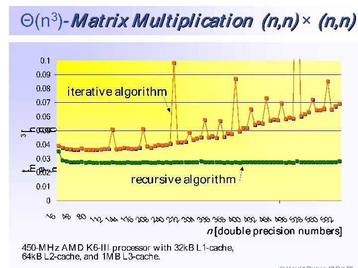
Towards faster matrix multiplication… (Blocked version) • Advantages – – Exploit locality using blocking Do not assume that each access to memory is O(1) Can be extended to multiple levels of cache Usually the fastest algorithm after tuning. • Disadvantages – Needs tuning every time it runs on a new machine. – Usually “s” is a voodoo parameter that is unknown.

Cache - Aware Matrix Multiplication BBLOCK-M ULT(A -MULT (A, B, C, n) 11 for ¬ 11 to for ii¬ to n/ n/ ss 22 do ¬ 11 to do for jj¬ to n/ n/ ss 33 do ¬ 11 to do for kk¬ to n/ n/ ss 44 do RD-M ULT(A -MULT (Aikik, B , Bkjkj, C , Cijij, s) do OORD Voodoo! s • Tune s so that A ik, Bkj, and Cij just fit into cache ? s = Z ( ) s • If n > s, then n 3 2 ( ) = ( ) ( Q n n s s L) = n 3 L Z. ( ( n ) ) • Optimal [HK 81]. © Harald Prokop 18 Oct 99 10

Cache Oblivious

Algorithms for External Memory

Computer P = Processor C = Cache M = Main Memory P C . . . M . . . Secondary Storage (Hard Disks)

Storage Capacity typical capacity (bytes) 1015 1013 1011 109 electronic secondary electronic main magnetic optical disks online tape nearline offline tape & tape optical disks 107 from Gray & Reuter (2002) 105 cache 103 10 -9 10 -6 10 -3 1 103 access time (sec)

Storage Cost 104 cache 102 dollars/MB from Gray & Reuter (2002) 100 electronic main electronic secondary online tape magnetic optical disks nearline tape & optical disks offline tape 10 -2 10 -4 10 -9 10 -6 10 -3 1 103 access time (sec)

Disk Access Time • Block X Request Block in Memory • Time = Seek Time + Rotational Delay + Transfer Time + Other Typical Numbers (for random block access) Seek Time = 10 ms Rot Delay = 4 ms (7200 rpm) transfer rate = 50 MB/sec Other = CPU time to access delays+ Contention for controllers Contention for Bus Multiple copies of the same data

Rules for EM Algorithms • Sequential IO is cheap compared to Random IO • 1 kb block – Seq : 1 ms – Random : 20 ms • The difference becomes smaller and smaller as the block size becomes larger.

The DAM Model • Count the number of IOs. • Explicitly control which Blocks are in memory. • Two level memory model. • Notation: • M = Size of memory. • B = size of disk block. • N = size of data. Question: How many block transfers for one scan of the data set?

Problem • Mergesort – How many Block IOs does it need to sort N numbers (when the size of the data is extremely large compared to M) • Can we do better?

External Memory Sorting • Penny Sort Competition 40 GB , 433 million records, 1541 seconds on a 614$ Linux/AMD system

EM Sorting • Two pass external memory merge sort. O(M) input: chunk 0 chunk 1 chunk 2 chunk 3 chunk 4 chunk 5 chunk 6 chunk 7 chunk 8 k=O(M/B) … run 0 run 1 run 2 run n … buffers B B k-merger run 0123 B … …

The CO Memory Model • Cache-oblivious memory model – Reason about two-level, but prove results for unknown multilevel memory models – Parameters B and M are unknown, thus optimized for all levels of memory hierarchy • B = L , M = Z?

Matrix Transpose: DAM n CO • What is the number of blocks you need to move in a transpose of a large matrix? – In DAM – In CO

Static Searches • Only for balanced binary trees • Assume there are no insertions and deletions • Only searches • Can we speed up such seaches?

What is a layout? • Mapping of nodes of a tree to the Memory • Different kinds of layouts – – In-order Post-order Pre-order Van Emde Boas • Main Idea : Store Recursive subtrees in contiguous memory

Example of Van Emde Boas

Another View

Theoretical Guarantees? • Cache Complexity Q(n) = O( ) • Work Complexity W(n) = O(log n) From Prokop’s Thesis

In Practice? ?

In Practice II

In Practice! • Matrix Operations by Morton Ordering , David S. Wise (Cache oblivious Practical Matrix operation results) • Bender, Duan, Wu (Cache oblivious dictionaries) • Rahman, Cole, Raman (CO B-Trees)

Known Optimal Results • Matrix Multiplication • Matrix Transpose • n-point FFT • LUP Decomposition • Sorting • Searching

Other Results Known Priority Q List Ranking Tree Algos Directed BFS/DFS Undirected BFS MSF

Introduction to Streaming Algorithms

Brain Teaser • Let P = { 1. . . n }. Let P’ = P {x} – x in P • Paul shows Carole elements from P’ • Carole can only use O(log n) bits memory to answer the question in the end. Now what about P’’?

Streaming Algorithms • Data that computers are being asked to process is growing astronomically. • Infeasible to store • If I cant store the data I am looking at, how do I compute a summary of this data?

Another Brain Teaser • Given a set of numbers in a large array. • In one pass, decide if some item is in majority (assume you only have constant size memory to work with). 2 9 9 9 7 6 4 9 9 9 3 9 N = 12; item 9 is majority Courtesy : Subhash Suri

Misra-Gries Algorithm • A counter and an ID. (‘ 82) – If new item is same as stored ID, increment counter. – Otherwise, decrement the counter. – If counter 0, store new item with count = 1. • If counter > 0, then its item is the only candidate for majority. 2 9 9 9 7 6 4 9 9 9 3 9 ID 2 2 9 9 4 4 9 9 count 1 0 1 2

Data Stream Algorithms • Majority and Frequent are examples of data stream algorithms. • Data arrives as an online sequence x 1, x 2, …, potentially infinite. • Algorithm processes data in one pass (in given order) • Algorithm’s memory is significantly smaller than input data • Summarize the data: compute useful patterns

Streaming Data Sources – – – – – Internet traffic monitoring New Computer Graphics hardware Web logs and click streams Financial and stock market data Retail and credit card transactions Telecom calling records Sensor networks, surveillance RFID Instruction profiling in microprocessors Data warehouses (random access too expensive).

FFT

Fast Fourier Transform: Applications • Applications. – Optics, acoustics, quantum physics, telecommunications, control systems, signal processing, speech recognition, data compression, image processing. – DVD, JPEG, MP 3, MRI, CAT scan. – Numerical solutions to Poisson's equation. The FFT is one of the truly great computational developments of this [20 th] century. It has changed the face of science and engineering so much that it is not an exaggeration to say that life as we know it would be very different without the FFT. -Charles van Loan

Fast Fourier Transform: Brief History • Gauss (1805, 1866). Analyzed periodic motion of asteroid Ceres. • Runge-König (1924). Laid theoretical groundwork. • Danielson-Lanczos (1942). Efficient algorithm. • Cooley-Tukey (1965). Monitoring nuclear tests in Soviet Union and tracking submarines. Rediscovered and popularized FFT. • Importance not fully realized until advent of digital computers.

Polynomials: Coefficient Representation • Polynomial. [coefficient representation] • Add: O(n) arithmetic operations. • Evaluate: O(n) using Horner's method. • Multiply (convolve): O(n 2) using brute force.

Polynomials: Point-Value Representation • Fundamental theorem of algebra. [Gauss, Ph. D thesis] A degree n polynomial with complex coefficients has n complex roots. • Corollary. A degree n-1 polynomial A(x) is uniquely specified by its evaluation at n distinct values of x. y yj = A(xj) xj x

Polynomials: Point-Value Representation • Polynomial. [point-value representation] • Add: O(n) arithmetic operations. • Multiply: O(n), but need 2 n-1 points. • Evaluate: O(n 2) using Lagrange's formula.

Converting Between Two Polynomial Representations • Tradeoff. Fast evaluation or fast multiplication. We want both! Representation Multiply Evaluate Coefficient O(n 2) O(n) Point-value O(n) O(n 2) • Goal. Make all ops fast by efficiently converting between two representations. coefficient representation point-value representation

Converting Between Two Polynomial Representations: Brute Force • Coefficient to point-value. Given a polynomial a 0 + a 1 x +. . . + an-1 xn-1, evaluate it at n distinct points x 0, . . . , xn-1. O(n 2) for matrix-vector multiply O(n 3) for Gaussian elimination Vandermonde matrix is invertible iff x i distinct • Point-value to coefficient. Given n distinct points x 0, . . . , xn-1 and values y 0, . . . , yn-1, find unique polynomial a 0 + a 1 x +. . . + an-1 xn-1 that has given values at given points.

Coefficient to Point-Value Representation: Intuition • Coefficient to point-value. Given a polynomial a 0 + a 1 x +. . . + an-1 xn 1, evaluate it at n distinct points x , . . . , x. 0 n-1 • Divide. Break polynomial up into even and odd powers. – A(x) = a 0 + a 1 x + a 2 x 2 + a 3 x 3 + a 4 x 4 + a 5 x 5 + a 6 x 6 + a 7 x 7. – Aeven(x) = a 0 + a 2 x + a 4 x 2 + a 6 x 3. – Aodd (x) = a 1 + a 3 x + a 5 x 2 + a 7 x 3. – A(-x) = Aeven(x 2) + x Aodd(x 2). – A(-x) = Aeven(x 2) - x Aodd(x 2). • Intuition. Choose two points to be 1. – A(-1) = Aeven(1) + 1 Aodd(1). Can evaluate polynomial of degree n – A(-1) = Aeven(1) - 1 Aodd(1). at 2 points by evaluating two polynomials of degree ½n at 1 point.

Coefficient to Point-Value Representation: Intuition • Coefficient to point-value. Given a polynomial a 0 + a 1 x +. . . + an-1 xn 1, evaluate it at n distinct points x , . . . , x. 0 n-1 • Divide. Break polynomial up into even and odd powers. – A(x) = a 0 + a 1 x + a 2 x 2 + a 3 x 3 + a 4 x 4 + a 5 x 5 + a 6 x 6 + a 7 x 7. – Aeven(x) = a 0 + a 2 x + a 4 x 2 + a 6 x 3. – Aodd (x) = a 1 + a 3 x + a 5 x 2 + a 7 x 3. – A(-x) = Aeven(x 2) + x Aodd(x 2). – A(-x) = Aeven(x 2) - x Aodd(x 2). • Intuition. Choose four points to be 1, i. – A(-1) = Aeven(-1) + 1 Aodd( 1). – A(-1) = Aeven(-1) - 1 Aodd(-1). Can evaluate polynomial of degree n at 4 points by evaluating two polynomials – A(-i) = Aeven(-1) + i Aodd(-1). of degree ½n at 2 points. – A(-i) = Aeven(-1) - i Aodd(-1).

Discrete Fourier Transform • Coefficient to point-value. Given a polynomial a 0 + a 1 x +. . . + an-1 xn 1, evaluate it at n distinct points x , . . . , x. 0 n-1 • Key idea: choose xk = k where is principal nth root of unity. Discrete Fourier transform Fourier matrix Fn

Roots of Unity • Def. An nth root of unity is a complex number x such that xn = 1. • • Fact. The nth roots of unity are: 0, 1, …, n-1 where = e 2 i / n. Pf. ( k)n = (e 2 i k / n) n = (e i ) 2 k = (-1) 2 k = 1. • • Fact. The ½nth roots of unity are: 0, 1, …, n/2 -1 where = e 4 i / n. Fact. 2 = and ( 2)k = k. 2 = 1 = i 3 1 n=8 4 = 2 = -1 0 = 1 7 5 6 = 3 = -i

Fast Fourier Transform • Goal. Evaluate a degree n-1 polynomial A(x) = a 0 +. . . + an-1 xn-1 at its nth roots of unity: 0, 1, …, n-1. • Divide. Break polynomial up into even and odd powers. – Aeven(x) = a 0 + a 2 x + a 4 x 2 + … + an/2 -2 x(n-1)/2. – Aodd (x) = a 1 + a 3 x + a 5 x 2 + … + an/2 -1 x(n-1)/2. – A(x) = Aeven(x 2) + x Aodd(x 2). • Conquer. Evaluate degree Aeven(x) and Aodd(x) at the ½nth roots of unity: 0, 1, …, n/2 -1. • Combine. – A( k+n) = Aeven( k) + k Aodd( k), 0 k < n/2 – A( k+n/2) = Aeven( k) - k Aodd( k), 0 k < n/2 k+n/2 = - k k = ( k)2 = ( k+n/2)2

FFT Algorithm fft(n, a 0, a 1, …, an-1) { if (n == 1) return a 0 (e 0, e 1, …, en/2 -1) FFT(n/2, a 0, a 2, a 4, …, an-2) (d 0, d 1, …, dn/2 -1) FFT(n/2, a 1, a 3, a 5, …, an-1) for k = k yk+n/2 } 0 to n/2 - 1 { e 2 ik/n e k + k d k e k - k d k return (y 0, y 1, …, yn-1) }

FFT Summary • Theorem. FFT algorithm evaluates a degree n-1 polynomial at each of the nth roots of unity in O(n log n) steps. assumes n is a power of 2 • Running time. T(2 n) = 2 T(n) + O(n) T(n) = O(n log n) coefficient representation point-value representation

Point-Value to Coefficient Representation: Inverse DFT • Goal. Given the values y 0, . . . , yn-1 of a degree n-1 polynomial at the n points 0, 1, …, n-1, find unique polynomial a 0 + a 1 x +. . . + an-1 xn-1 that has given values at given points. Inverse DFT Fourier matrix inverse (Fn)-1

Inverse FFT • Claim. Inverse of Fourier matrix is given by following formula.

Inverse FFT: Proof of Correctness • • Claim. Fn and Gn are inverses. Pf. summation lemma • Summation lemma. Let be a principal nth root of unity. Then • Pf. – If k is a multiple of n then k = 1 sums to n. – Each nth root of unity k is a root of xn - 1 = (x - 1) (1 + x 2 +. . . + xn-1). – if k 1 we have: 1 + k(2) +. . . + k(n-1) = 0 sums to 0. ▪

Inverse FFT: Algorithm ifft(n, a 0, a 1, …, an-1) { if (n == 1) return a 0 (e 0, e 1, …, en/2 -1) FFT(n/2, a 0, a 2, a 4, …, an-2) (d 0, d 1, …, dn/2 -1) FFT(n/2, a 1, a 3, a 5, …, an-1) for k = k yk+n/2 } 0 to n/2 - 1 { e-2 ik/n (ek + k dk) / n (ek - k dk) / n return (y 0, y 1, …, yn-1) }

• Inverse FFT Summary Theorem. Inverse FFT algorithm interpolates a degree n-1 polynomial given values at each of the nth roots of unity in O(n log n) steps. assumes n is a power of 2 O(n log n) coefficient representation O(n log n) point-value representation

Polynomial Multiplication • Theorem. Can multiply two degree n-1 polynomials in O(n log n) steps. coefficient representation FFT coefficient representation O(n log n) inverse FFT point-value multiplication O(n) O(n log n)

FFT in Practice • Fastest Fourier transform in the West. [Frigo and Johnson] – Optimized C library. – Features: DFT, DCT, real, complex, any size, any dimension. – Won 1999 Wilkinson Prize for Numerical Software. – Portable, competitive with vendor-tuned code. • Implementation details. – Instead of executing predetermined algorithm, it evaluates your hardware and uses a special-purpose compiler to generate an optimized algorithm catered to "shape" of the problem. – Core algorithm is nonrecursive version of Cooley-Tukey radix 2 FFT. – O(n log n), even for prime sizes. Reference: http: //www. fftw. org

More on FFT 0, 4, 2, 6, 1, 5, 3, 7

FFT

Parallel FFT a 0 a 1 a 2 a 3 a 4 a 5 a 6 a 7 y 0 y 1 y 2 y 3 y 4 y 5 y 6 y 7

Integer Multiplication • Integer multiplication. Given two n bit integers a = an-1 … a 1 a 0 and b = bn-1 … b 1 b 0, compute their product c = a b. • Convolution algorithm. – Form two polynomials. – Note: a = A(2), b = B(2). – Compute C(x) = A(x) B(x). – Evaluate C(2) = a b. – Running time: O(n log n) complex arithmetic steps. • Theory. [Schönhage-Strassen 1971] O(n log log n) bit operations. • Practice. [GNU Multiple Precision Arithmetic Library] GMP proclaims to be "the fastest bignum library on the planet. " It uses brute force, Karatsuba, and FFT, depending on the size of n.