Advanced Algorithm Design and Analysis Lecture 3 SW

Advanced Algorithm Design and Analysis (Lecture 3) SW 5 fall 2004 Simonas Šaltenis E 1 -215 b simas@cs. aau. dk AALG, lecture 3, © Simonas Šaltenis, 2004

Text-search Algorithms n Goals of the lecture: n n n Naive text-search algorithm and its analysis; Rabin-Karp algorithm and its analysis; Knuth-Morris-Pratt algorithm ideas; Boyer-Moore-Horspool algorithm and its analysis. Comparison of the advantages and disadvantages of the different text-search algorithms. AALG, lecture 3, © Simonas Šaltenis, 2004 2

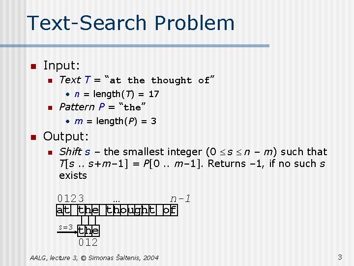
Text-Search Problem n Input: n Text T = “at the thought of” • n = length(T) = 17 n Pattern P = “the” • m = length(P) = 3 n Output: n Shift s – the smallest integer (0 £ s £ n – m) such that T[s. . s+m– 1] = P[0. . m– 1]. Returns – 1, if no such s exists 0123 … n-1 at the thought of s=3 the 012 AALG, lecture 3, © Simonas Šaltenis, 2004 3

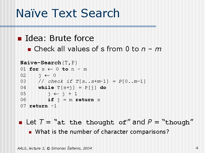
Naïve Text Search n Idea: Brute force n Check all values of s from 0 to n – m Naive-Search(T, P) 01 for s ¬ 0 to n – m 02 j ¬ 0 03 // check if T[s. . s+m– 1] = P[0. . m– 1] 04 while T[s+j] = P[j] do 05 j ¬ j + 1 06 if j = m return s 07 return – 1 n Let T = “at the thought of” and P = “though” n What is the number of character comparisons? AALG, lecture 3, © Simonas Šaltenis, 2004 4

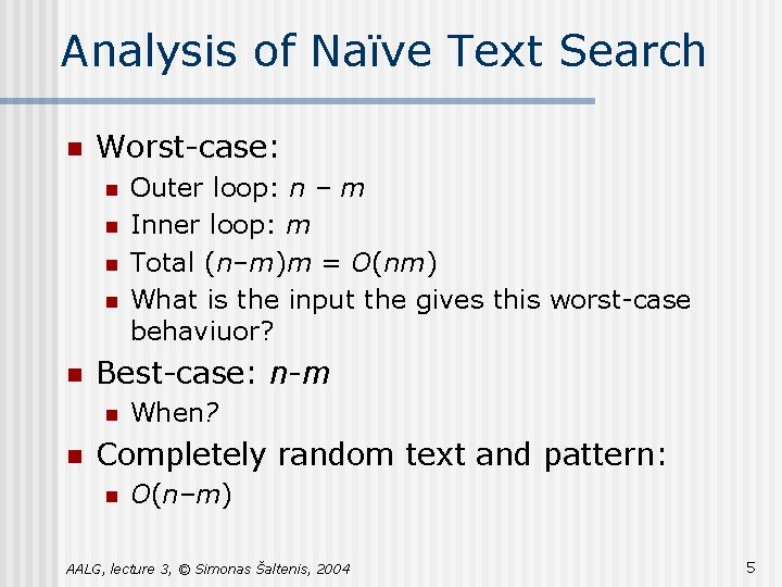
Analysis of Naïve Text Search n Worst-case: n n n Best-case: n-m n n Outer loop: n – m Inner loop: m Total (n–m)m = O(nm) What is the input the gives this worst-case behaviuor? When? Completely random text and pattern: n O(n–m) AALG, lecture 3, © Simonas Šaltenis, 2004 5

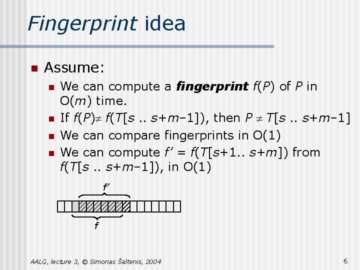
Fingerprint idea n Assume: n n We can compute a fingerprint f(P) of P in O(m) time. If f(P)¹ f(T[s. . s+m– 1]), then P ¹ T[s. . s+m– 1] We can compare fingerprints in O(1) We can compute f’ = f(T[s+1. . s+m]) from f(T[s. . s+m– 1]), in O(1) f’ f AALG, lecture 3, © Simonas Šaltenis, 2004 6

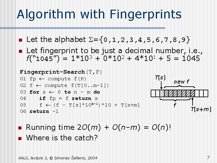
Algorithm with Fingerprints n Let the alphabet S={0, 1, 2, 3, 4, 5, 6, 7, 8, 9} n Let fingerprint to be just a decimal number, i. e. , f(“ 1045”) = 1*103 + 0*102 + 4*101 + 5 = 1045 Fingerprint-Search(T, P) 01 fp ¬ compute f(P) 02 f ¬ compute f(T[0. . m– 1]) 03 for s ¬ 0 to n – m do 04 if fp = f return s 05 f ¬ (f – T[s]*10 m-1)*10 + T[s+m] 06 return – 1 n n T[s] new f f T[s+m] Running time 2 O(m) + O(n–m) = O(n)! Where is the catch? AALG, lecture 3, © Simonas Šaltenis, 2004 7

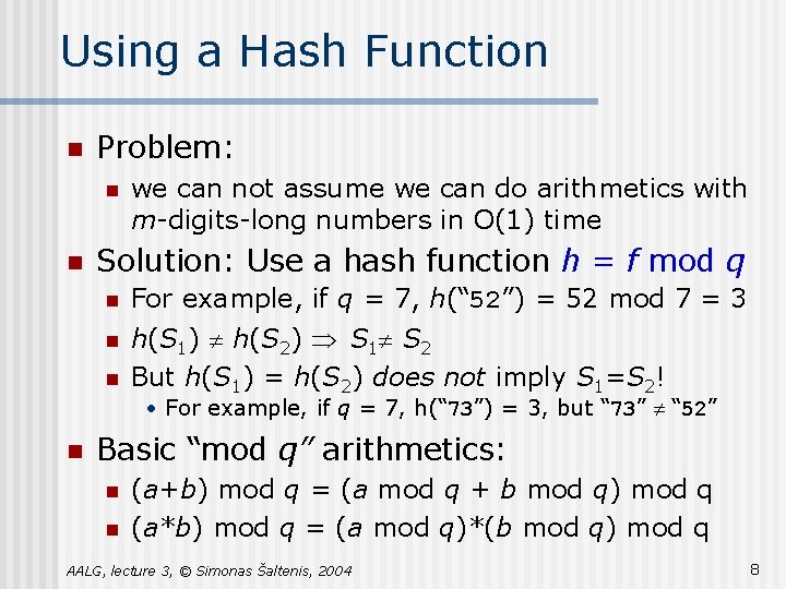
Using a Hash Function n Problem: n n we can not assume we can do arithmetics with m-digits-long numbers in O(1) time Solution: Use a hash function h = f mod q n For example, if q = 7, h(“ 52”) = 52 mod 7 = 3 n h(S 1) ¹ h(S 2) Þ S 1¹ S 2 But h(S 1) = h(S 2) does not imply S 1=S 2! n • For example, if q = 7, h(“ 73”) = 3, but “ 73” ¹ “ 52” n Basic “mod q” arithmetics: n n (a+b) mod q = (a mod q + b mod q) mod q (a*b) mod q = (a mod q)*(b mod q) mod q AALG, lecture 3, © Simonas Šaltenis, 2004 8

Preprocessing and Stepping n Preprocessing: n n fp = P[m-1] + 10*(P[m-2] + 10*(P[m-3]+ … … + 10*(P[1] + 10*P[0])…)) mod q In the same way compute ft from T[0. . m-1] Example: P = “ 2531”, q = 7, what is fp? Stepping: n n n ft = (ft – T[s]*10 m-1 mod q)*10 + T[s+m]) mod q 10 m-1 mod q can be computed once in the preprocessing Example: Let T[…] = “ 5319”, q = 7, what is the corresponding ft? T[s] new ft ft AALG, lecture 3, © Simonas Šaltenis, 2004 T[s+m] 9

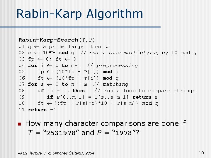
Rabin-Karp Algorithm Rabin-Karp-Search(T, P) 01 q ¬ a prime larger than m 02 c ¬ 10 m-1 mod q // run a loop multiplying by 10 mod q 03 fp ¬ 0; ft ¬ 0 04 for i ¬ 0 to m-1 // preprocessing 05 fp ¬ (10*fp + P[i]) mod q 06 ft ¬ (10*ft + T[i]) mod q 07 for s ¬ 0 to n – m // matching 08 if fp = ft then // run a loop to compare strings 09 if P[0. . m-1] = T[s. . s+m-1] return s 10 ft ¬ ((ft – T[s]*c)*10 + T[s+m]) mod q 11 return – 1 n How many character comparisons are done if T = “ 2531978” and P = “ 1978”? AALG, lecture 3, © Simonas Šaltenis, 2004 10

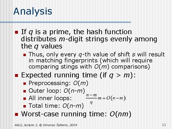
Analysis n If q is a prime, the hash function distributes m-digit strings evenly among the q values n n Expected running time (if q > m): n n n Thus, only every q-th value of shift s will result in matching fingerprints (which will require comparing stings with O(m) comparisons) Preprocessing: O(m) Outer loop: O(n-m) All inner loops: Total time: O(n-m) Worst-case running time: O(nm) AALG, lecture 3, © Simonas Šaltenis, 2004 11

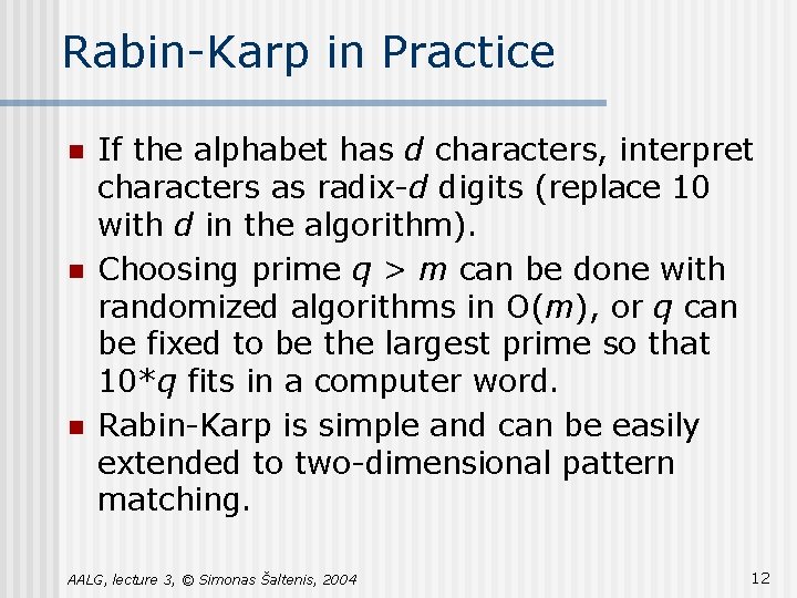
Rabin-Karp in Practice n n n If the alphabet has d characters, interpret characters as radix-d digits (replace 10 with d in the algorithm). Choosing prime q > m can be done with randomized algorithms in O(m), or q can be fixed to be the largest prime so that 10*q fits in a computer word. Rabin-Karp is simple and can be easily extended to two-dimensional pattern matching. AALG, lecture 3, © Simonas Šaltenis, 2004 12

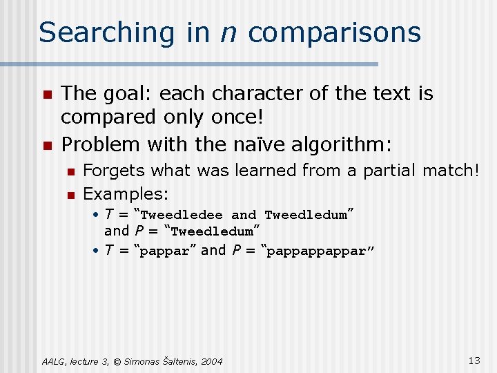
Searching in n comparisons n n The goal: each character of the text is compared only once! Problem with the naïve algorithm: n n Forgets what was learned from a partial match! Examples: • T = “Tweedledee and Tweedledum” and P = “Tweedledum” • T = “pappar” and P = “pappappappar” AALG, lecture 3, © Simonas Šaltenis, 2004 13

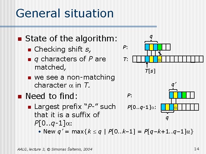
General situation n n q State of the algorithm: Checking shift s, q characters of P are matched, we see a non-matching character a in T. Need to find: n Largest prefix “P-” such that it is a suffix of P[0. . q-1]a: P: T: a T[s] q’ P: P[0. . q-1]a: a q • New q’ = max{k £ q | P[0. . k– 1] = P[q–k+1. . q– 1]a} AALG, lecture 3, © Simonas Šaltenis, 2004 14

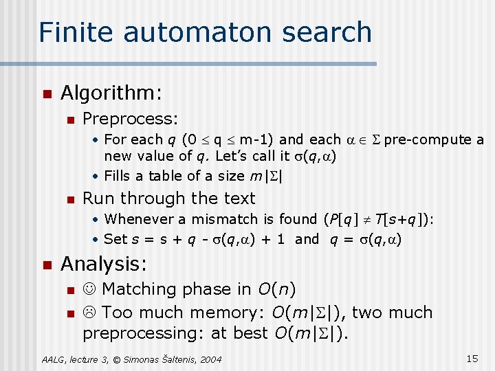
Finite automaton search n Algorithm: n Preprocess: • For each q (0 £ q £ m-1) and each a Î S pre-compute a new value of q. Let’s call it s(q, a) • Fills a table of a size m|S| n Run through the text • Whenever a mismatch is found (P[q] ¹ T[s+q]): • Set s = s + q - s(q, a) + 1 and q = s(q, a) n Analysis: n n Matching phase in O(n) Too much memory: O(m|S|), two much preprocessing: at best O(m|S|). AALG, lecture 3, © Simonas Šaltenis, 2004 15

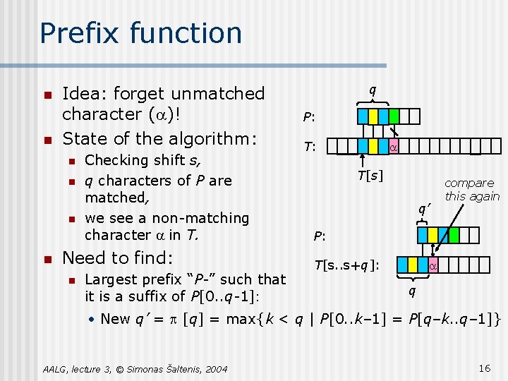
Prefix function n n Idea: forget unmatched character (a)! State of the algorithm: n n Checking shift s, q characters of P are matched, we see a non-matching character a in T. Need to find: n Largest prefix “P-” such that it is a suffix of P[0. . q-1]: q P: T: a T[s] q’ compare this again P: T[s. . s+q]: a q • New q’ = p [q] = max{k < q | P[0. . k– 1] = P[q–k. . q– 1]} AALG, lecture 3, © Simonas Šaltenis, 2004 16

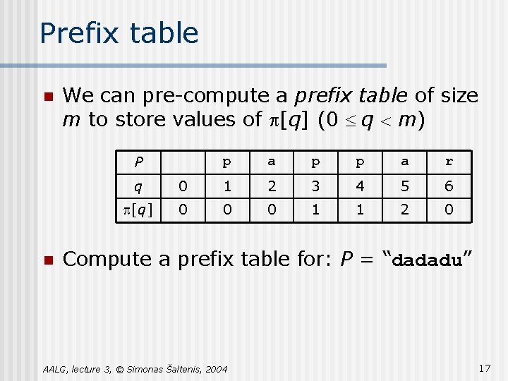
Prefix table n We can pre-compute a prefix table of size m to store values of p[q] (0 £ q < m) P n p a p p a r q 0 1 2 3 4 5 6 p[q] 0 0 0 1 1 2 0 Compute a prefix table for: P = “dadadu” AALG, lecture 3, © Simonas Šaltenis, 2004 17

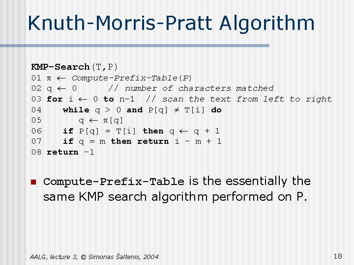
Knuth-Morris-Pratt Algorithm KMP-Search(T, P) 01 p ¬ Compute-Prefix-Table(P) 02 q ¬ 0 // number of characters matched 03 for i ¬ 0 to n-1 // scan the text from left to right 04 while q > 0 and P[q] ¹ T[i] do 05 q ¬ p[q] 06 if P[q] = T[i] then q ¬ q + 1 07 if q = m then return i – m + 1 08 return – 1 n Compute-Prefix-Table is the essentially the same KMP search algorithm performed on P. AALG, lecture 3, © Simonas Šaltenis, 2004 18

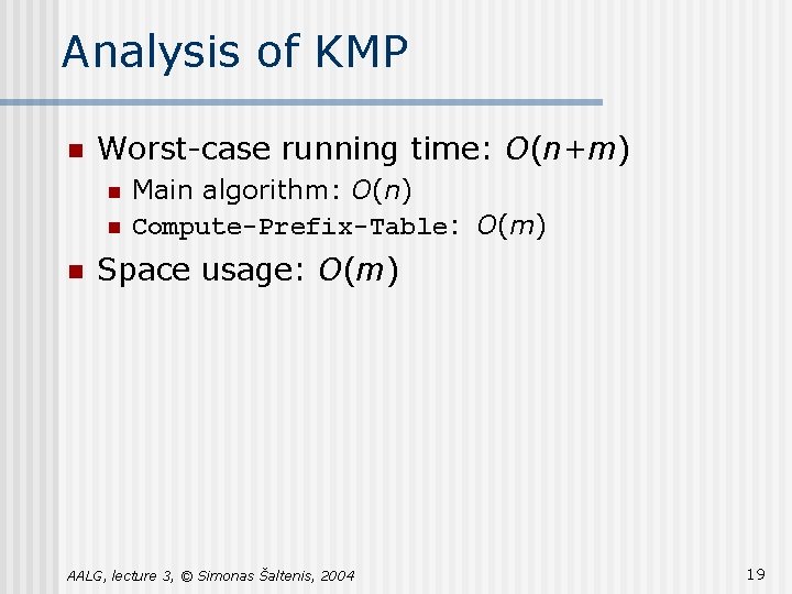
Analysis of KMP n Worst-case running time: O(n+m) n n n Main algorithm: O(n) Compute-Prefix-Table: O(m) Space usage: O(m) AALG, lecture 3, © Simonas Šaltenis, 2004 19

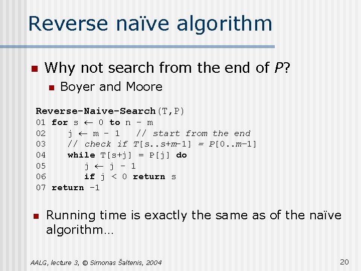
Reverse naïve algorithm n Why not search from the end of P? n Boyer and Moore Reverse-Naive-Search(T, P) 01 for s ¬ 0 to n – m 02 j ¬ m – 1 // start from the end 03 // check if T[s. . s+m– 1] = P[0. . m– 1] 04 while T[s+j] = P[j] do 05 j ¬ j - 1 06 if j < 0 return s 07 return – 1 n Running time is exactly the same as of the naïve algorithm… AALG, lecture 3, © Simonas Šaltenis, 2004 20

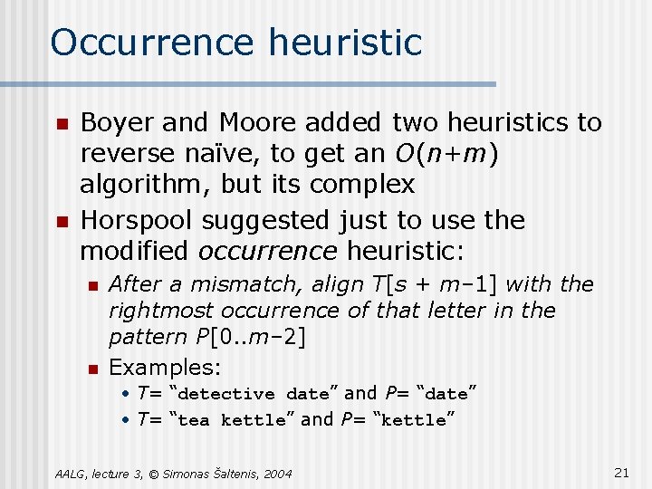
Occurrence heuristic n n Boyer and Moore added two heuristics to reverse naïve, to get an O(n+m) algorithm, but its complex Horspool suggested just to use the modified occurrence heuristic: n n After a mismatch, align T[s + m– 1] with the rightmost occurrence of that letter in the pattern P[0. . m– 2] Examples: • T= “detective date” and P= “date” • T= “tea kettle” and P= “kettle” AALG, lecture 3, © Simonas Šaltenis, 2004 21

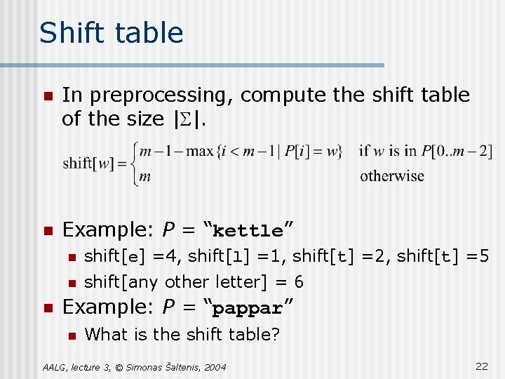
Shift table n In preprocessing, compute the shift table of the size |S|. n Example: P = “kettle” n n shift[e] =4, shift[l] =1, shift[t] =2, shift[t] =5 n shift[any other letter] = 6 Example: P = “pappar” n What is the shift table? AALG, lecture 3, © Simonas Šaltenis, 2004 22

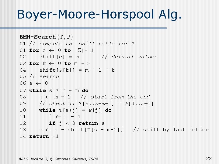
Boyer-Moore-Horspool Alg. BMH-Search(T, P) 01 // compute the shift table for P 01 for c ¬ 0 to |S|- 1 02 shift[c] = m // default values 03 for k ¬ 0 to m - 2 04 shift[P[k]] = m – 1 - k 05 // search 06 s ¬ 0 07 while s £ n – m do 08 j ¬ m – 1 // start from the end 09 // check if T[s. . s+m– 1] = P[0. . m– 1] 10 while T[s+j] = P[j] do 11 j ¬ j - 1 12 if j < 0 return s 13 s ¬ s + shift[T[s + m– 1]] // shift by last letter 14 return – 1 AALG, lecture 3, © Simonas Šaltenis, 2004 23

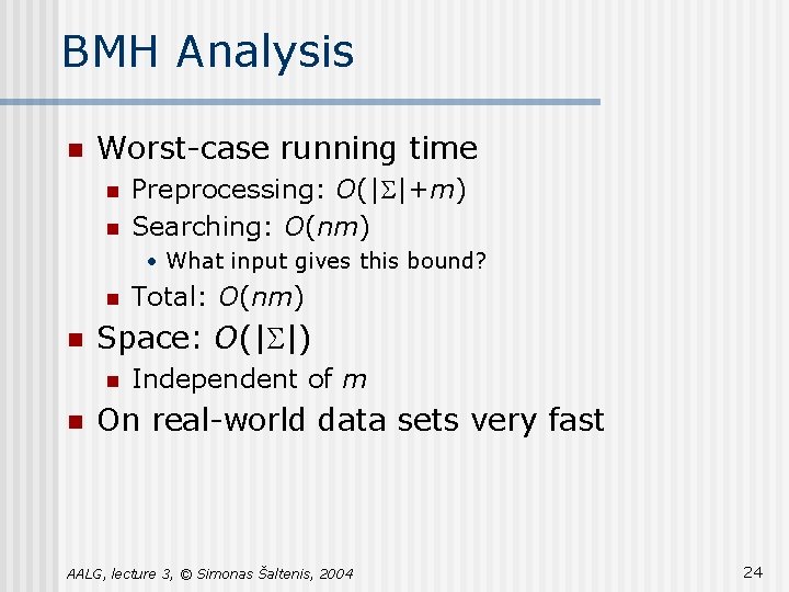
BMH Analysis n Worst-case running time n n Preprocessing: O(|S|+m) Searching: O(nm) • What input gives this bound? n n Space: O(|S|) n n Total: O(nm) Independent of m On real-world data sets very fast AALG, lecture 3, © Simonas Šaltenis, 2004 24

Comparison n Let’s compare the algorithms. Criteria: n Worst-case running time • Preprocessing • Searching n n n Expected running time Space used Implementation complexity AALG, lecture 3, © Simonas Šaltenis, 2004 25