Advancd Regional Prediction System ARPS Ming Xue mxueou

Advancd Regional Prediction System (ARPS) Ming Xue mxue@ou. edu School of Meteorology and Center for Analysis and Prediction of Storms University of Oklahoma

Model Dynamics, Equations and Numerical Formualtions See PDF file

Initial Condition

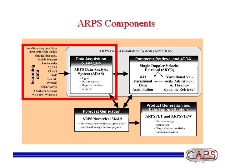
ARPS Components

Ways to Initialize ARPS • Idealized, single sounding • Interpolation from GFS, Eta, RUC, etc • ADAS

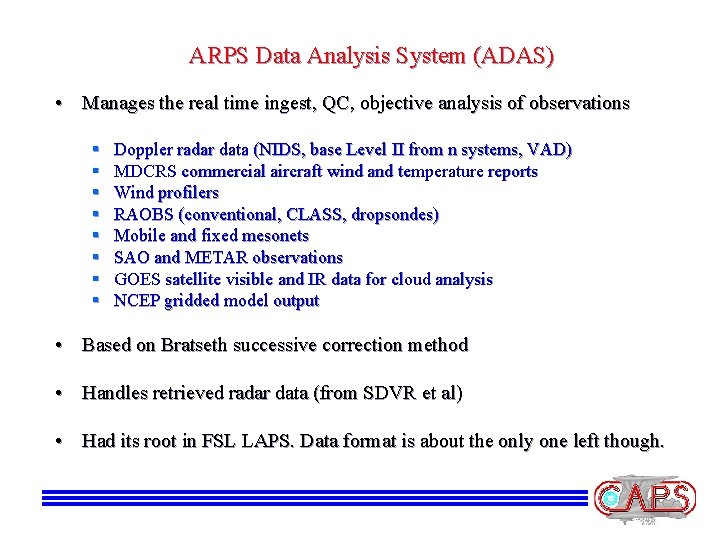
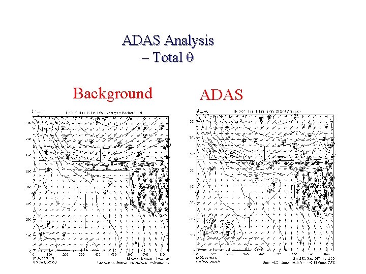
ARPS Data Analysis System (ADAS) • Manages the real time ingest, QC, objective analysis of observations § § § § Doppler radar data (NIDS, base Level II from n systems, VAD) MDCRS commercial aircraft wind and temperature reports Wind profilers RAOBS (conventional, CLASS, dropsondes) Mobile and fixed mesonets SAO and METAR observations GOES satellite visible and IR data for cloud analysis NCEP gridded model output • Based on Bratseth successive correction method • Handles retrieved radar data (from SDVR et al) • Had its root in FSL LAPS. Data format is about the only one left though.

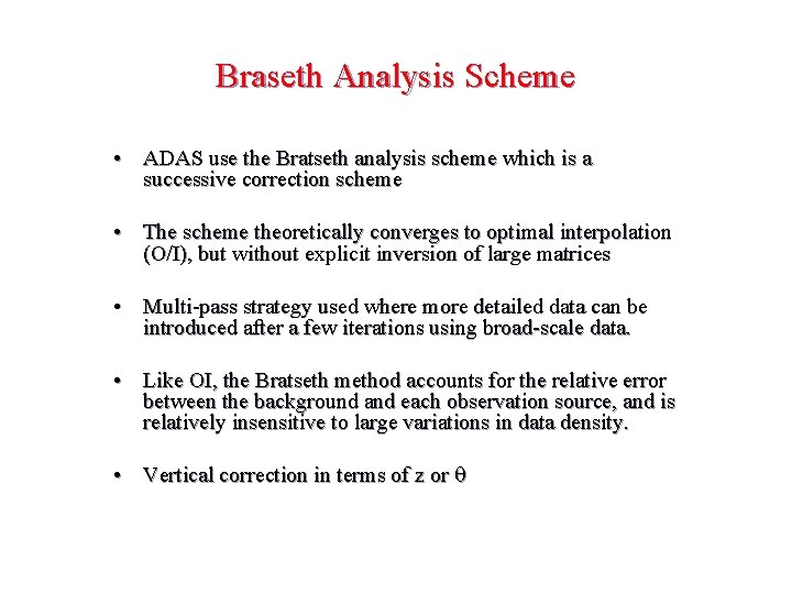
Braseth Analysis Scheme • ADAS use the Bratseth analysis scheme which is a successive correction scheme • The scheme theoretically converges to optimal interpolation (O/I), but without explicit inversion of large matrices • Multi-pass strategy used where more detailed data can be introduced after a few iterations using broad-scale data. • Like OI, the Bratseth method accounts for the relative error between the background and each observation source, and is relatively insensitive to large variations in data density. • Vertical correction in terms of z or q

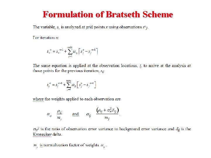
Formulation of Bratseth Scheme

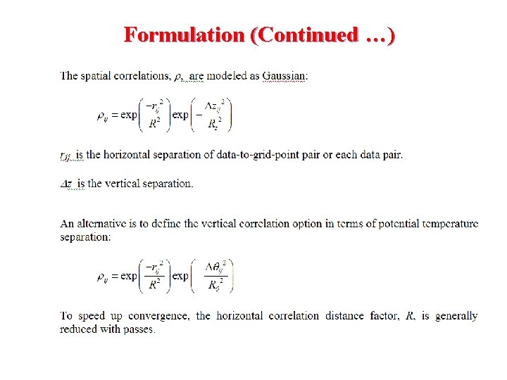
Formulation (Continued …)

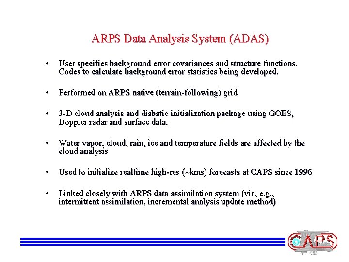
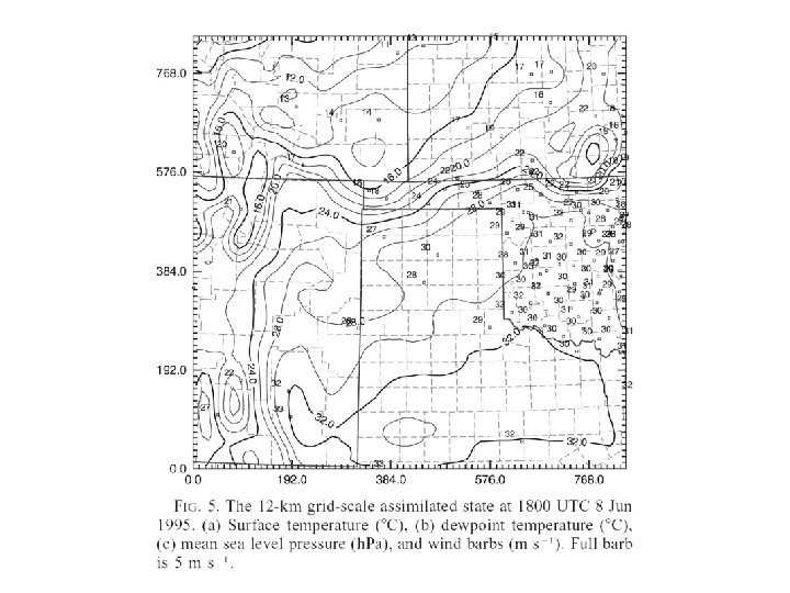
ARPS Data Analysis System (ADAS) • User specifies background error covariances and structure functions. Codes to calculate background error statistics being developed. • Performed on ARPS native (terrain-following) grid • 3 -D cloud analysis and diabatic initialization package using GOES, Doppler radar and surface data. • Water vapor, cloud, rain, ice and temperature fields are affected by the cloud analysis • Used to initialize realtime high-res (~kms) forecasts at CAPS since 1996 • Linked closely with ARPS data assimilation system (via, e. g. , intermittent assimilation, incremental analysis update method)

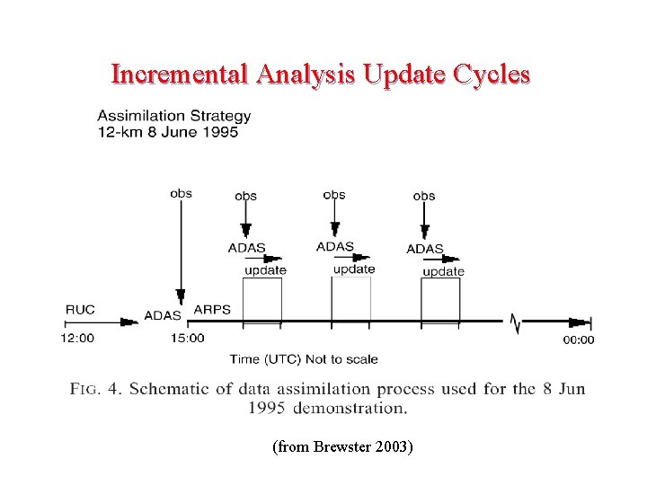
Incremental Analysis Update Cycles (from Brewster 2003)

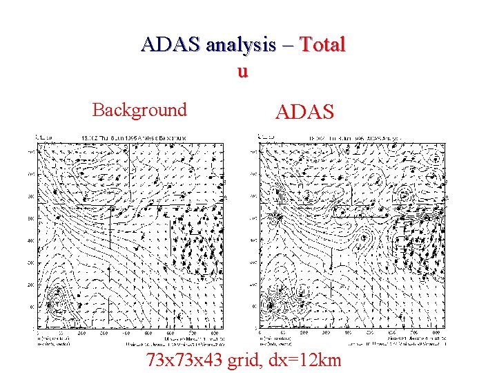
ADAS analysis – Total u Background ADAS 73 x 43 grid, dx=12 km

ADAS Analysis – Total q Background ADAS

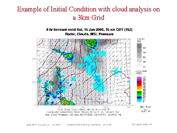
Example of Initial Condition with cloud analysis on a 3 km Grid

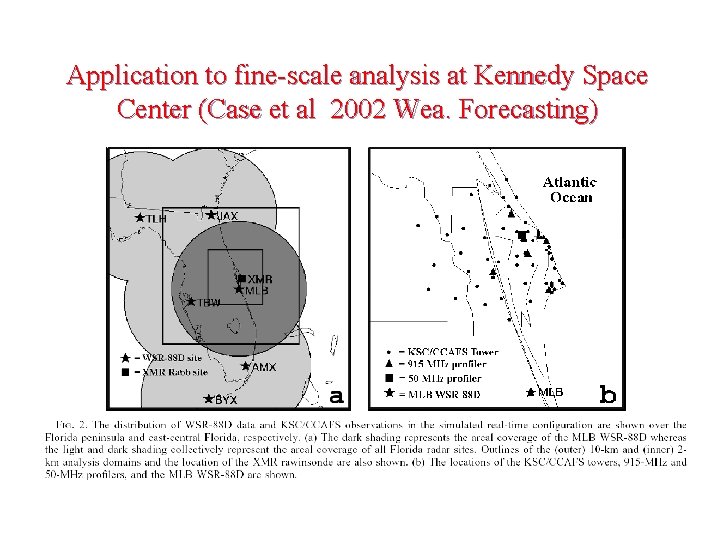
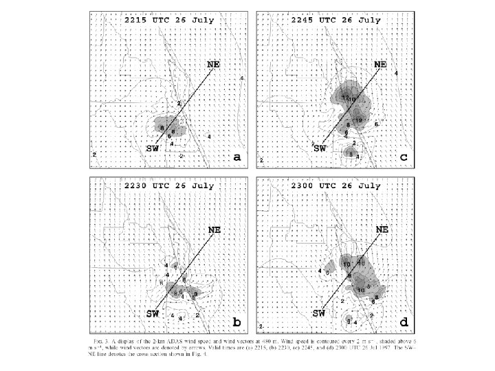
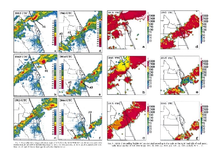
Application to fine-scale analysis at Kennedy Space Center (Case et al 2002 Wea. Forecasting)

Boundary Conditions • Lateral Boundary Conditions § Rigid, zero-gradient, periodic § Open/radiative LBC (only applied to normal velocity) § Externally (can be from the same model) forced o o Davies-type relaxation zone, arbitrary width w not forced variables (e. g. , water) not found in exbc are excluded from relaxation – zero gradient is usually applied Ensure same terrain at nesting boundaries § Carpenter (1982) – radiation BC with external forcing(? ) o Carpenter, K. M. , 1982: Note on radiation conditions for the lateral boundaries of limited-area numerical models. Quart. J. Roy. Meteor. Soc. , 108, 717 -719.

Vertical Boundary Condition • Radiation top BC based on cosine Fourier transform (Klemp and Durran 1983) § periodicity requirement at the top relaxed § Still based on linearized equations – difficult to apply to large domain • Upper boundary sponge/absorbing layer § relaxation to coarse grid/external model solution in the layer § or relaxation to the mean state • Rigid, zero-gradient and periodic top-bottom BC • Semi-slip lower BC

Stratiform Clouds and Precipitation • Microphysics parameterization for grid-scale precipitation • Can be used together with cumulus parameterization schemes • Option to allow condensation at subsatuation (<100% RH) § helps retaining clouds in IC for large grid spacing § improves surface temperature forecast at low-resolution by introducing clouds earlier • Sedimentation term treated implicitly or using time splitting

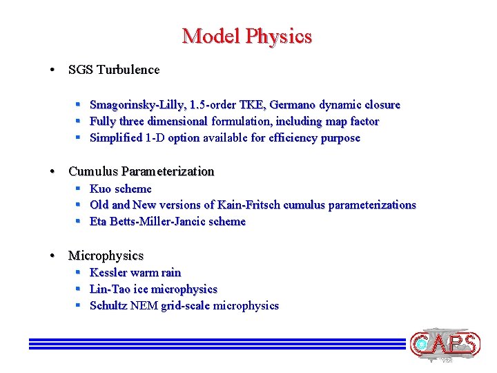
Model Physics • SGS Turbulence § Smagorinsky-Lilly, 1. 5 -order TKE, Germano dynamic closure § Fully three dimensional formulation, including map factor § Simplified 1 -D option available for efficiency purpose • Cumulus Parameterization § Kuo scheme § Old and New versions of Kain-Fritsch cumulus parameterizations § Eta Betts-Miller-Jancic scheme • Microphysics § § § Kessler warm rain Lin-Tao ice microphysics Schultz NEM grid-scale microphysics

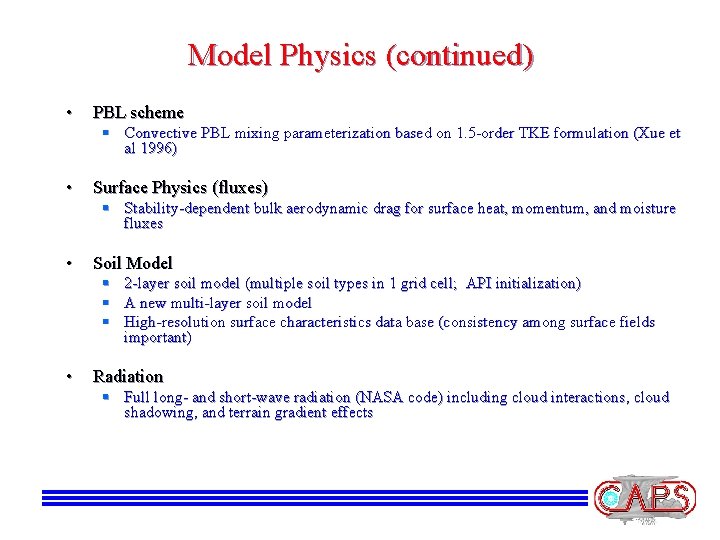
Model Physics (continued) • PBL scheme § Convective PBL mixing parameterization based on 1. 5 -order TKE formulation (Xue et al 1996) • Surface Physics (fluxes) § Stability-dependent bulk aerodynamic drag for surface heat, momentum, and moisture fluxes • Soil Model § § § • 2 -layer soil model (multiple soil types in 1 grid cell; API initialization) A new multi-layer soil model High-resolution surface characteristics data base (consistency among surface fields important) Radiation § Full long- and short-wave radiation (NASA code) including cloud interactions, cloud shadowing, and terrain gradient effects

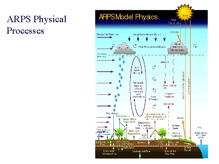
ARPS Physical Processes

Subgrid Scale Fluxes (Land surface, surface layer, PBL and SGS turbulence) See PDF file

Radiation

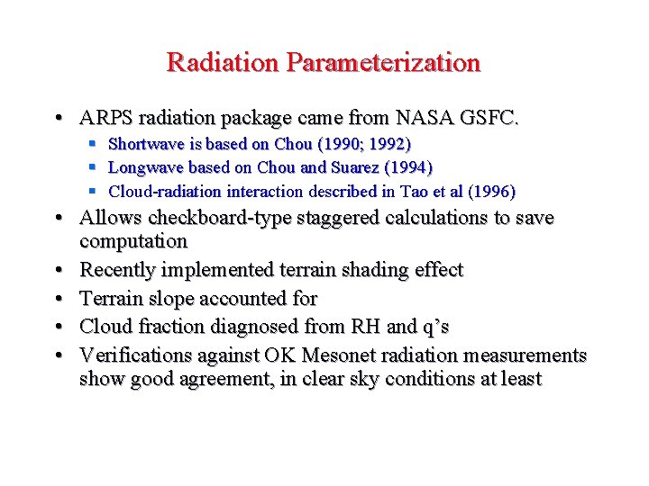
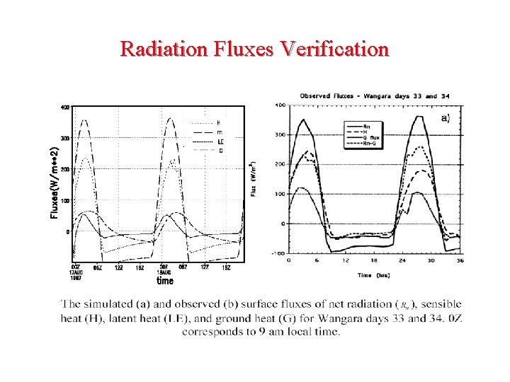
Radiation Parameterization • ARPS radiation package came from NASA GSFC. § Shortwave is based on Chou (1990; 1992) § Longwave based on Chou and Suarez (1994) § Cloud-radiation interaction described in Tao et al (1996) • Allows checkboard-type staggered calculations to save computation • Recently implemented terrain shading effect • Terrain slope accounted for • Cloud fraction diagnosed from RH and q’s • Verifications against OK Mesonet radiation measurements show good agreement, in clear sky conditions at least

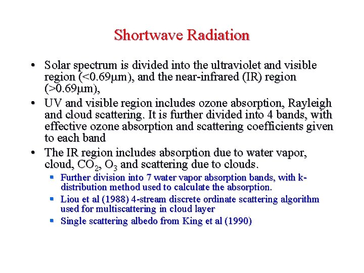
Shortwave Radiation • Solar spectrum is divided into the ultraviolet and visible region (<0. 69 mm), and the near-infrared (IR) region (>0. 69 mm), • UV and visible region includes ozone absorption, Rayleigh and cloud scattering. It is further divided into 4 bands, with effective ozone absorption and scattering coefficients given to each band • The IR region includes absorption due to water vapor, cloud, CO 2, O 3 and scattering due to clouds. § Further division into 7 water vapor absorption bands, with kdistribution method used to calculate the absorption. § Liou et al (1988) 4 -stream discrete ordinate scattering algorithm used for multiscattering in cloud layer § Single scattering albedo from King et al (1990)

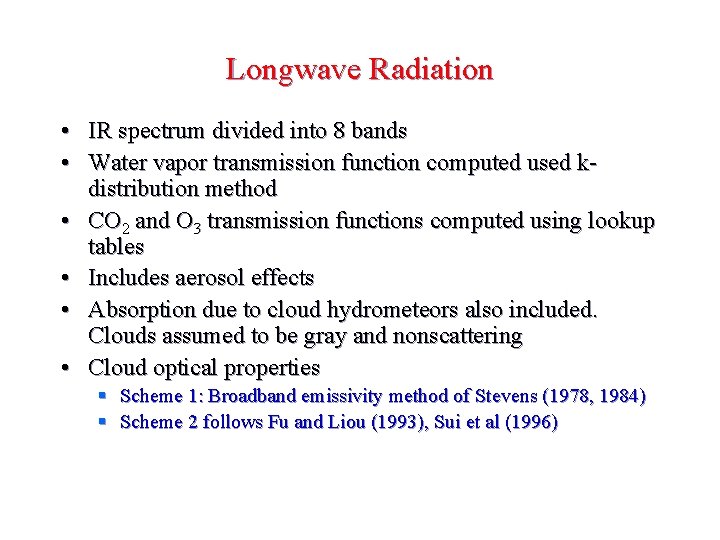
Longwave Radiation • IR spectrum divided into 8 bands • Water vapor transmission function computed used kdistribution method • CO 2 and O 3 transmission functions computed using lookup tables • Includes aerosol effects • Absorption due to cloud hydrometeors also included. Clouds assumed to be gray and nonscattering • Cloud optical properties § Scheme 1: Broadband emissivity method of Stevens (1978, 1984) § Scheme 2 follows Fu and Liou (1993), Sui et al (1996)

Radiation Fluxes Verification

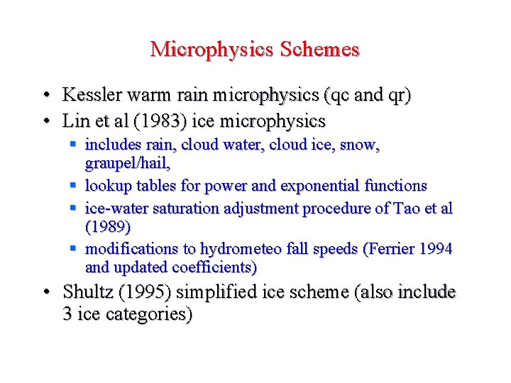
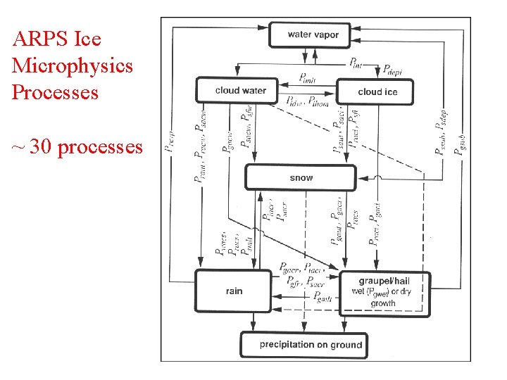
Microphysics Schemes • Kessler warm rain microphysics (qc and qr) • Lin et al (1983) ice microphysics § includes rain, cloud water, cloud ice, snow, graupel/hail, § lookup tables for power and exponential functions § ice-water saturation adjustment procedure of Tao et al (1989) § modifications to hydrometeo fall speeds (Ferrier 1994 and updated coefficients) • Shultz (1995) simplified ice scheme (also include 3 ice categories)

ARPS Ice Microphysics Processes ~ 30 processes

Accumulated Precipitation from 1977 Del City Supercell Storms with warmrain and ice microphysics

Simulation of 1977 Del City Supercell Storms with warmrain and ice microphysics

Convective Parameterization

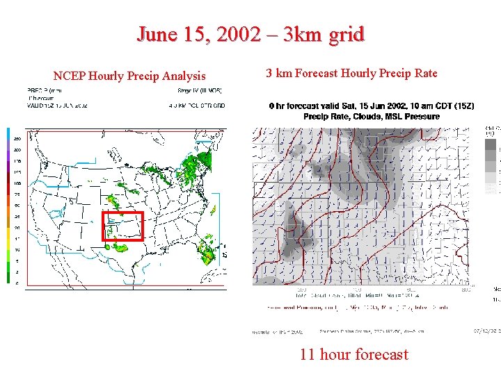
Convective Clouds and Precipitation • At high resolutions (=< 3 km), use ‘explicit’ microphysics, hopefully the model can resolve the convection well • Cumulus parameterization schemes § Kuo scheme § Old and new Kain-Fritch schemes § Betts-Miller-Janjic scheme § New K-F scheme used most

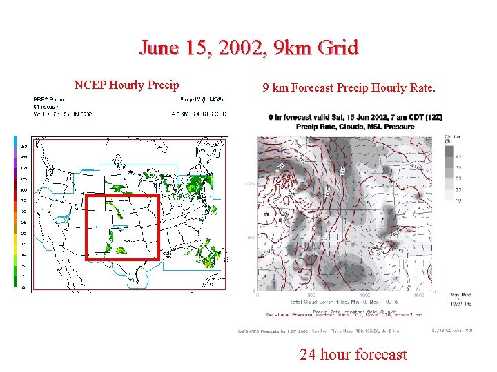
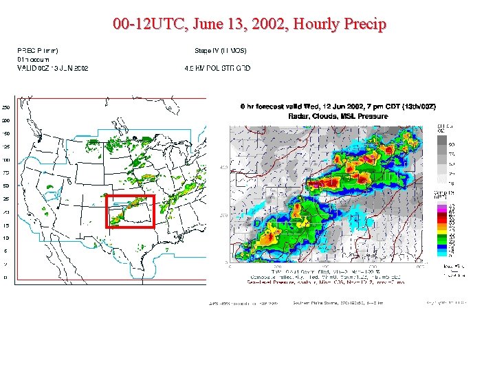
Use of Cumulus Scheme • K-F scheme used most • New K-F scheme using at 27 and 9 km during IHOP realtime forecast • BMJ scheme tends to produce much smoother precipitation field • Cold pool important for propagation of convective systems over the plains • Triggering of spurious propagating precipitation pattern observed during IHOP

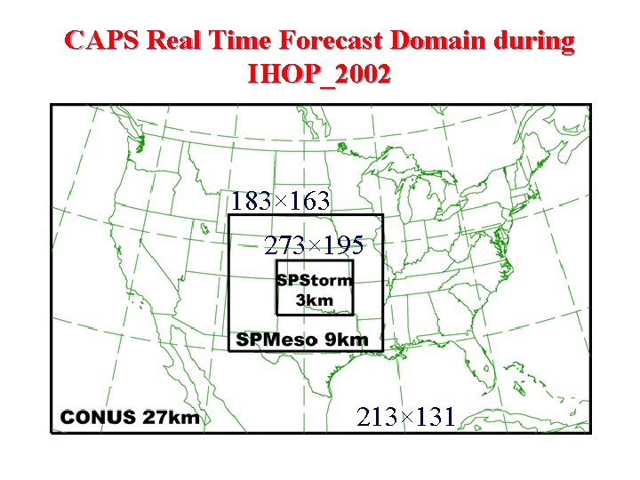
CAPS Real Time Forecast Domain during IHOP_2002 183× 163 273× 195 213× 131

June 15, 2002, 9 km Grid NCEP Hourly Precip 9 km Forecast Precip Hourly Rate. 24 hour forecast

June 15, 2002 – 3 km grid NCEP Hourly Precip Analysis 3 km Forecast Hourly Precip Rate 11 hour forecast

00 -12 UTC, June 13, 2002, Hourly Precip